Model
Model Overview
From 0.03% to 87%: The Truth Behind the Efficiency Gap
Imagine a gene integration system where success rates can vary by nearly 3000-fold under different conditions. This isn't an experimental error—it’s a black box waiting to be opened.
In our GenOMe system, one-to-one means that one pair of attB and attP sites recombines once through Bxb1 integrase to form one integration event.
Traditional genetic engineering relies on trial and error, but we asked:
- Which step truly limits efficiency?
- Why is two-to-two deletion so much harder than one-to-one insertion?
- Can we mathematically predict optimal conditions instead of blind testing?
Our answer: Build an interpretable, predictive five-layer integration model.
The Efficiency Gap at a Glance
| System Type | Traditional Mode A | Ready-to-Integrate Mode B | Efficiency Gain |
|---|---|---|---|
| One-to-one | ~0.57% | - | - |
| Two-to-two | ~0.05% | 79–87% | 1600-fold |
A single variable change produces a three-order-of-magnitude leap — this is the core mystery our model explains.
Modeling Strategy: Dissecting the Black Box Layer by Layer
We decomposed the Bxb1 gene integration system into five modelable biological layers, peeling away complexity like an onion:


Model1(M1): Transcriptional Dynamics and Induction Window Optimization
Quantifies how arabinose initiates Bxb1 gene transcription and the dynamics of mRNA production and degradation.
M2 - Translation Layer: The Protein Accumulation Race
Calculates how long it takes for Bxb1 protein to reach effective concentration and when it begins to lose activity.
M3 - Chromosomal Layer: The Hidden Major Bottleneck
Models how ssAP forms attB sites on the chromosome — the system’s most fragile step.
Mechanism Breakdown: ssAP (single-strand annealing protein) must:
- Be taken up by cells (efficiency ~10–30%)
- Find the replication fork spatiotemporal window
- Successfully anneal with the lagging strand
- Avoid degradation or dilution
The multiplication of these four steps results in overall success rate < 1%.
M4 - Recombination Layer: The Two-Site Coordination Challenge
Quantifies how Bxb1 recognizes and recombines two attB sites, and why longer fragments reduce efficiency.
M5 - Experimental Assistant: From Mechanism to Practical Tool

Transforms parameters from the first four layers into a lookup-table success rate predictor for experiment design.
Three Core Discoveries
Discovery 1: The Real Bottleneck Isn’t Where You Think
Most would assume low Bxb1 protein concentration causes poor efficiency. But the model reveals:
- Intracellular Bxb1 reaches 200–400 nM (μM range)
- In vitro experiments need only 10–50 nM for efficient recombination
- So why is efficiency still low in living cells?
The answer lies in M3: randomness of attB site formation is the true killer.
- Single ssAP integration probability into chromosome < 1%
- Success rate strongly depends on chromosomal position:
- Near oriC: ~0.6%
- Near terC: ~0.03% (20-fold difference!)
Position Effect Formula: P(d) ≈ 0.6% × e−0.0007d, where d = distance from oriC (kb).
Discovery 2: The Mechanistic Cost of Two-to-Two
At the same chromosomal position (oriC-proximal), we compared:
- One-to-one: ~0.57% success rate
- Two-to-two: ~0.05% success rate
Why the 10-fold difference? The model provides the answer:
The fundamental mechanism complexity differs, not just a probability multiplication:
Success_one-to-one = P₀ × [modification factors]
≈ 0.001066 × φtot × fgc × flocus × distance_factor × …
≈ 0.57%
Success_two-to-two = P₀_dual × [same modification factors]
≈ (P₀ / 15–20) × φtot × fgc × flocus × distance_factor × …
≈ 0.05%
Why is P₀_dual so much smaller? Two-to-two deletion requires:
- Two independent ssAP integration events both succeed
- Spatial coordination between distant chromosomal sites
- Synchronized recombination at both attB sites
- Any single failure aborts the entire process
Intuitive understanding: It's like needing to successfully thread two needles at once while they're moving—even if you're skilled at threading one needle (one-to-one), doing two simultaneously in coordination is fundamentally harder, not just twice as hard.
Mechanistic complexity multiplier: Two-to-two is 15-20 times harder than one-to-one
Discovery 3: Skip the Bottleneck, Efficiency Soars to 80%+
When using Ready-to-Integrate Mode B (linear DNA with pre-built attB sites):
| Fragment Length | Measured Success | Model Prediction | Error |
|---|---|---|---|
| 1039 bp | 87.5% | 87.6% | +0.1% |
| 1605 bp | 79.0% | 79.3% | +0.3% |
| 1613 bp | 80.0% | 79.1% | −0.9% |
Average prediction error < 0.4%
The model not only predicts accurately but also explains why:
- Bypasses the M3 bottleneck (no need for ssAP to form attB)
- M4 recombination becomes the dominant step, but remains efficient in the 1-2 kb range
- Bxb1 concentration reaches effective range within 30 minutes
Model Validation: Data Speaks
We calibrated the model using three length anchor points (1039/1605/1613 bp):
Mean Absolute Error (MAE) = 0.37%
Maximum deviation < 1%
Covers practical range 1.0-1.6 kb
All predictions include 95% confidence intervals, with extrapolation regions (>4 kb, extreme GC%) clearly marked.
How to Read This Model?
Choose different reading paths based on your needs:
I want to use it quickly
→ Jump directly to M5 Experimental Design Assistant
Input your fragment parameters and get success rate predictions from the lookup table.
I want to understand why efficiency is low
→ Focus on M3 vs M4 Comparative Analysis
See where the bottleneck truly lies.
I want complete mechanistic understanding
→ Read sequentially M1 → M2 → M3 → M4 → M5
Trace the complete process from induction to integration.
I want to improve or adapt this model
→ Consult parameter tables and calibration guidelines for each layer.
All assumptions and limitations are explicitly stated.
What Does This Model Tell Us?
- Low efficiency isn't due to insufficient Bxb1, but because attB formation is too difficult.
- Chromosomal position effects are physical limitations that traditional mode cannot avoid.
- Two-to-two deletion is inherently harder than one-to-one insertion (mechanistic complexity).
- Mode B system bypasses the bottleneck, maintaining ≥80% efficiency for 1–2 kb fragments.
- Simple conditions suffice: 300–400 nM Bxb1, 30 minutes reaches the concentration plateau.
Extended Implications of the Model
Can this modeling framework be transferred to other systems?
Yes! This five-layer architecture applies to any gene editing system requiring:
- Induced expression (M1–M2)
- Chromosomal site marking (M3)
- Sequence-specific recombination (M4)
Examples include:
- Other integrases: Cre-loxP, FLP-FRT, ΦC31
- CRISPR systems: Use M3 to model sgRNA delivery, M4 to model Cas9 cleavage efficiency
- Transposon systems: Tn5, Tn7, etc.
Insights for Modern Gene Editing
The model reveals that "delivery bottleneck > reaction kinetics" — a principle explaining why:
- In vitro assembled RNPs (CRISPR) outperform plasmid expression
- Electroporated DNA is more stable than chemical transformation
- Viral vectors dominate in eukaryotic cells
The underlying logic is the same: bypass random intracellular synthesis/marking processes by directly delivering functional molecules.
Ready to Dive Deeper?
This is not just a mathematical model, but a complete roadmap from gene expression to genome rewriting.
Choose your path and start exploring
Have questions about modeling? Want to see raw data? Click the sections to begin your journey!
Model1(M1): Transcriptional Dynamics of Bxb1 Expression
Model Scope
The M1 model describes the mRNA dynamics of ssAP (single-strand annealing protein) and Bxb1 integrase under various induction regimes.
- The transcriptional outputs mg(t) provide direct input for M2 protein accumulation.
- Together, M1 and M2 determine whether proteins reach functional steady states required for M3 (attB formation) and M4 (recombination).
A key feature of M1 is its ability to resolve induction time windows, including the effect of cooling periods where transcription is reduced but not fully terminated.
Mathematical Formulation
mRNA dynamics are governed by:
$$ \frac{dm_g}{dt} = \beta_g \cdot I_g(t) - d_{m,g} m_g, \quad g \in \{ \text{Bxb1, ssAP} \} $$
where:
- mg(t): mRNA concentration (μM)
- βg: transcription rate (μM/min)
- dm,g=ln(2)/t1/2: degradation constant (1/min), defined by half-life
- Ig(t): induction function, varying with experimental design
Model Parameters
| Name | Definition | Value [unit] | Reference |
|---|---|---|---|
| βssAP | Transcription rate of ssAP | 0.15 [μM/min] | Estimated from promoter strength [1] |
| βBxb1 | Transcription rate of Bxb1 | 0.10 [μM/min] | Estimated from promoter strength [1] |
| βBxb1-J23105 | Transcription rate of Bxb1 under promoter J23105 | 0.04 [μM/min] | iGEM Registry [3] |
| t1/2,ssAP | mRNA half-life of ssAP | 7.0 [min] | Literature [2] |
| t1/2,Bxb1 | mRNA half-life of Bxb1 | 6.9 [min] | Literature [2] |
| t1/2,Bxb1-J23105 | mRNA half-life of Bxb1-J23105 | 6.8 [min] | Literature [2] |
| dm,ssAP | Degradation constant of ssAP mRNA | 0.099 [1/min] | Derived from half-life [2] |
| dm,Bxb1 | Degradation constant of Bxb1 mRNA | 0.100 [1/min] | Derived from half-life [2] |
| dm,Bxb1-J23105 | Degradation constant of Bxb1-J23105 mRNA | 0.102 [1/min] | Derived from half-life [2] |
| γ | Residual transcription ratio during cooling | 0.1 | Literature [5] |
| tinduce,ssAP | Induction time for ssAP | 45 [min] | Experimental condition |
| tinduce,Bxb1 | Induction time for Bxb1 | 240 [min] | Experimental condition |
| tinduce,J23105 | Induction time for J23105 promoter | 240 [min] | Experimental condition |
| tcool,ssAP | Cooling time for ssAP | 10 [min] | Experimental setting |
For ssAP, we explicitly incorporated a cooling phase to reflect reduced transcriptional activity:
$ I(t) = \begin{cases} 1, & 0 \le t < 45 \quad \text{(full induction)} \\ \gamma, & 45 \le t < 55 \quad \text{(cooling, residual activity)} \\ 0, & t \ge 55 \quad \text{(fully off)} \end{cases} $
with γ = 0.1, representing 10% residual transcriptional efficiency during cooling on ice [4].
Analytical solutions follow canonical forms:
- Continuous induction (I = 1):
$$ m(t) = \frac{\beta}{d_m} \left(1 - e^{-d_m t}\right) $$ - Switch-off (I = 0):
$$ m(t) = m(t_{\text{off}}) e^{-d_m (t - t_{\text{off}})} $$ - Steady-state level:
$$ m_{\text{steady}} = \frac{\beta}{d_m} $$
These are standard analytical solutions [5] obtained by solving the first-order ODE for mRNA dynamics.
Simulation Results
-
ssAP (45 min induction + 10 min cooling)
- mRNA rose rapidly to a peak of ~1.43 μM at 45 min.
- During the cooling phase, transcription was not fully halted but reduced to 10% activity, slowing decay.
- By 120 min, mRNA levels approached baseline, illustrating a transient profile.

-
Bxb1 (inducible, 240 min with L-arabinose)
- mRNA reached 95% of steady state within ~30 min, then maintained a plateau for 4 h.
- This demonstrates long-term sustained supply consistent with Bxb1’s catalytic role.

-
Bxb1 (constitutive expression, promoter J23105)
- Steady-state mRNA concentration stabilized at ~0.109 μM, significantly lower than inducible conditions.
- Nevertheless, it provides a low but persistent baseline.

Conclusions and Experimental Guidance
- Conclusions:
- M1 captures distinct temporal regimes: transient (ssAP) vs. sustained (Bxb1).
- Protein bottlenecks arise not from insufficient magnitude but from induction cutoffs before steady-state.
- Cooling phases must be considered as low-efficiency transcriptional windows, not as complete shutdowns.
-
Guidance:
Extend ssAP induction to 45 min to align with its mRNA peak, accounting for residual transcription during cooling.
[1] Registry of Standard Biological Parts (iGEM). (n.d.). Promoter BBa_J23105. Retrieved from http://parts.igem.org/Part:BBa_J23105
[2] Bernstein, J. A., Khodursky, A. B., Lin, P. H., Lin-Chao, S., & Cohen, S. N. (2002). Global analysis of mRNA decay and abundance in Escherichia coli at single-gene resolution using two-color fluorescent DNA microarrays. PNAS, 99(15), 9697–9702. https://doi.org/10.1073/pnas.112318199
[3] Selinger, D. W., Saxena, R. M., Cheung, K. J., Church, G. M., & Rosenow, C. (2003). Global RNA half-life analysis in Escherichia coli reveals positional patterns of transcript degradation. Genome Research, 13(2), 216–223. https://doi.org/10.1101/gr.912603
[4] Phadtare, S., & Inouye, M. (2003). Cold shock response and cold shock proteins. Genes & Development, 17(8), 971–981. https://doi.org/10.1101/gad.1077503
[5] Alon, U. (2006). An Introduction to Systems Biology: Design Principles of Biological Circuits. Chapman & Hall/CRC.
Model2(M2): Translation Dynamics and Protein Accumulation
Model Scope
Building upon the transcriptional dynamics characterized in M1, the M2 model quantifies the accumulation of ssAP and Bxb1 proteins.
- The mRNA profiles from M1 serve as direct inputs for translation.
- Protein concentrations are the decisive factors for downstream steps: ssAP enabling attB formation (M3) and Bxb1 catalyzing attP × attB recombination (M4).
Thus, M2 serves as the critical bridge between gene expression and functional integration efficiency. Its role is to evaluate whether extended induction windows are sufficient to ensure proteins act within their effective functional windows.
Mathematical Formulation with Translation Delay
We start from the canonical mRNA–protein dynamics widely used in gene expression modeling.
(1) mRNA dynamics
$$ \frac{dm_g}{dt} = \beta_g I_g(t) - d_{m,g} m_g(t), \quad g \in \{\mathrm{Bxb1}, \mathrm{ssAP}\}. \quad [1][2] $$
This is a first–order linear ODE describing production at rate $\beta_g$ (controlled by induction function $I_g(t)$) and degradation at rate $d_{m,g}$. The analytical solution is obtained using the integrating factor method:
$$ m_g(t) = m_g(0)e^{-d_{m,g}t} + \int_0^t \beta_g I_g(s)e^{-d_{m,g}(t-s)}\, ds. \quad [1][2] $$
Special cases include:
-
Continuous induction, $I_g=1$, $m_g(0)=0$:
$$ m_g(t) = \frac{\beta_g}{d_{m,g}}(1 - e^{-d_{m,g}t}). \quad [1] $$ -
Switch-off at $t_{\mathrm{off}}$:
$$ m_g(t) = m_g(t_{\mathrm{off}}) e^{-d_{m,g}(t - t_{\mathrm{off}})}. \quad [1] $$ - Steady state: $$ m_{g,\mathrm{ss}} = \beta_g / d_{m,g}.\quad [1] $$
Moreover, the degradation constant is related to the mRNA half-life by $d_{m,g} = \ln 2 / t_{1/2}$, which in E. coli has been globally quantified to be on the order of a few minutes [5].
(2) Protein dynamics with translation delay
We incorporate an average translation/maturation delay $\tau$, such that fully functional proteins appear only after time $\tau$:
$$ \frac{dP_g}{dt} = k_{\mathrm{trans},g}\, m_g(t - \tau) - d^{\mathrm{eff}}_{p,g}\, P_g, \quad [3][4] $$
where the effective decay constant combines protein degradation and growth dilution:
$$ d^{\mathrm{eff}}_{p,g} \equiv k^{P}_{\mathrm{deg},g} + \mu. \quad [1][2] $$
The convention is $m_g(t - \tau) = 0$ for $t < \tau$.
(3) Analytical solutions (continuous induction example)
Assume $I_g(t) = 1$ with initial conditions $m_g(0) = P_g(0) = 0$.
-
mRNA solution
$$ m_g(t) = \frac{\beta_g}{d_{m,g}}\left(1 - e^{-d_{m,g}t}\right). \quad [1][2] $$ -
Protein solution with delay
- For $t < \tau$: $$ P_g(t) = 0. \quad [3][4] $$
- For $t \ge \tau$: $$ P_g(t) = \frac{k_{\mathrm{trans},g}\,\beta_g}{d_{m,g}\,d^{\mathrm{eff}}_{p,g}} \left(1 - e^{-d^{\mathrm{eff}}_{p,g}(t-\tau)}\right) - \frac{k_{\mathrm{trans},g}\,\beta_g}{d_{m,g}\left(d^{\mathrm{eff}}_{p,g}-d_{m,g}\right)} \left(e^{-d_{m,g}(t-\tau)} - e^{-d^{\mathrm{eff}}_{p,g}(t-\tau)}\right). \quad [3][4] $$
This expression shows that the protein dynamics are identical to the no-delay case, but shifted by $(t - \tau)$.
(4) Generalization
For switch-off or pulse induction with residual activity \(\gamma\), one substitutes the time-dependent \(I_g(t)\) into the mRNA solution and propagates it through the protein convolution. The closed form remains valid provided all terms are shifted by \((t-\tau)\) and \(d_p\) is replaced by dp,geff.
Protein removal is modeled through an effective decay constant \(d_{p,\mathrm{eff}}=d_p+\mu\), where \(\mu\) represents dilution due to cell growth and \(d_p\) denotes intrinsic protein degradation. In M2 we assume a constant \(\mu\), corresponding to balanced exponential growth, to keep the focus on transcription–translation–recombination dynamics. A burden-aware formulation \(\mu([\textit{Bxb1}])\) is introduced later as an optional extension.
| Name | Definition | Value [unit] | Reference |
|---|---|---|---|
| βssAP | Transcription rate of ssAP mRNA | 0.15 [μM/min] | Estimated from promoter strength [6] |
| βBxb1 | Transcription rate of Bxb1 mRNA (induced) | 0.10 [μM/min] | Estimated from promoter strength [6] |
| βBxb1-J23105 | Transcription rate of Bxb1 under J23105 promoter | 0.04 [μM/min] | iGEM Registry [6] |
| t1/2, mRNA, ssAP | mRNA half-life of ssAP | 7.0 [min] | Literature [7,8] |
| t1/2, mRNA, Bxb1 | mRNA half-life of Bxb1 | 6.9 [min] | Literature [7,8] |
| t1/2, mRNA, Bxb1-J23105 | mRNA half-life of Bxb1-J23105 | 6.8 [min] | Literature [7,8] |
| dm, ssAP | mRNA degradation constant of ssAP | 0.099 [1/min] | Calculated as ln2 / t1/2 [7,8] |
| dm, Bxb1 | mRNA degradation constant of Bxb1 | 0.100 [1/min] | Calculated as ln2 / t1/2 [7,8] |
| dm, Bxb1-J23105 | mRNA degradation constant of Bxb1-J23105 | 0.102 [1/min] | Calculated as ln2 / t1/2 [7,8] |
| ktrans, ssAP | Translation rate constant of ssAP | 0.50 [1/min] (baseline assumption) | Assumed unified value; later fitted [9,10] |
| ktrans, Bxb1 | Translation rate constant of Bxb1 | 0.20 [1/min] (baseline assumption) | Assumed unified value [9,10] |
| ktrans, Bxb1-J23105 | Translation rate constant of Bxb1 (J23105 promoter) | 0.20 [1/min] (baseline assumption) | Assumed unified value [9,10] |
| τ | Translation delay (initiation/maturation) | 2 [min] | Assumed; typical ribosome initiation + maturation delay [9] |
| t1/2, Protein, ssAP | Protein half-life of ssAP | 60 [min] | Literature: short-lived protein [11] |
| t1/2, Protein, Bxb1 | Protein half-life of Bxb1 | 960 [min] (16 h) | Literature: stable protein [11] |
| t1/2, Protein, Bxb1-J23105 | Protein half-life of Bxb1-J23105 | 960 [min] (16 h) | Literature: stable protein [11] |
| dp, ssAP | Protein degradation constant of ssAP | 0.012 [1/min] | Derived from half-life [11] |
| dp, Bxb1 | Protein degradation constant of Bxb1 | ≈ 0 [1/min] | Derived from half-life [11] |
| dp, Bxb1-J23105 | Protein degradation constant of Bxb1-J23105 | ≈ 0 [1/min] | Derived from half-life [11] |
| μ | Growth dilution rate | ~0.0116 [1/min] (Td=60 min) | Calculated as ln2 / Td |
| dpeff | Effective protein decay constant | $ d_p^{\text{eff}} = dp + \mu $ | Model definition |
Simulation Results
- ssAP (45 min induction + 10 min cooling)
- Protein concentration peaked at ~9.5 μM around 48 min.
- Levels declined to ~6 μM by 120 min due to degradation.
- The transient dynamic matches its role as a short-lived auxiliary factor.

- Bxb1 (inducible, 240 min with L-arabinose)
- Protein accumulated continuously, reaching ~42 μM at 240 min.
- Due to its long half-life (>16 h), Bxb1 maintained a near-plateau even after induction ceased.
- Represents long-term stable supply, ideal for recombination catalysis.

- Bxb1 (constitutive expression, promoter J23105, 240 min)
- Accumulated more slowly, reaching ~0.3 μM at 240 min.
- Despite lower levels, still sufficient to support recombination, serving as a baseline self-sufficient regime.

Biological Interpretation
Comparison with Literature
In vitro assays typically employ serine integrases at 200–400 nM, occasionally up to 1000 nM.
Our simulations predicted μM-range intracellular concentrations, one to two orders of magnitude higher.
This confirms that absolute protein abundance is not the limiting factor in vivo.
Temporal Considerations
The critical determinant is not whether proteins reach steady-state, but whether they are present at the right time window.
- ssAP must first bind to the oligo to generate attB sites.
-
Bxb1 then needs sufficient time to encounter both the newly formed attB and the pre-installed attP to catalyze recombination.
Because this step requires two-site coordination and may be limited by conformational accessibility, short induction leaves Bxb1 with too little opportunity to capture both sites.
Extending induction therefore increases the encounter probability within the effective reaction window, rather than merely raising overall abundance.
Role Differentiation
- ssAP: rapid accumulation and decay → transient support for attB formation.
- Bxb1: gradual but persistent accumulation → sustained catalytic supply, provided the induction window is long enough to cover the recombination step.
Dry–Wet Interaction and Design Decisions
Dry → Wet (Prediction to Guidance):
- Initial inductions (30 min ssAP, 2 h Bxb1) were predicted to leave proteins insufficiently aligned with their effective functional windows, restricting recombination efficiency.
- Based on M1–M2 integration, we recommended extending induction windows: ssAP to 45 min and Bxb1 to 4 h, ensuring transient ssAP action is captured and Bxb1 has enough time for dual-site encounters.
Wet → Dry (Feedback to Refinement):
- Experimental teams extended induction accordingly (ssAP: 30 → 45 min; Bxb1: 2 h → 4 h).
- Feedback from colony counts will recalibrate degradation constants and refine M2 protein predictions.
This cycle demonstrates how modeling can directly shape experimental protocols by moving beyond concentration magnitude and instead emphasizing the importance of temporal coordination and encounter probability.
Without this temporal adjustment, downstream recombination (M4) would systematically underestimate efficiency, despite protein abundance being non-limiting.
Conclusions and Experimental Guidance
Conclusions:
- Intracellular protein levels are already far above in vitro requirements, ruling out insufficiency as a bottleneck.
- The decisive factor is whether induction windows allow ssAP to generate attB and give Bxb1 adequate time to engage both attB and attP.
Experimental Guidance:
- Maintain ssAP induction for 45 min to align with its transient peak and attB formation.
- Extend Bxb1 induction to 4 h to maximize the probability of dual-site recombination events.
This adjustment ensures effective coordination of M3 and M4, improving recombination efficiency without requiring higher expression strength.
Graphics for Wiki/Publication
- Figure 1: Overlaid protein dynamics curves (ssAP transient, Bxb1 inducible plateau, Bxb1 constitutive slow rise).

- Figure 2: Flow diagram of Dry–Wet interaction: Model prediction → Experimental adjustment (longer induction) → Data feedback → Model refinement.

[1]Alon, U. (2006). An Introduction to Systems Biology: Design Principles of Biological Circuits. Chapman & Hall/CRC.
[2]Thattai, M., & van Oudenaarden, A. (2001). Intrinsic noise in gene regulatory networks. PNAS, 98(15), 8614–8619.https://doi.org/10.1073/pnas.151588598
[3]Monk, N. A. M. (2003). Oscillatory expression of Hes1, p53, and NF-κB driven by transcriptional time delays. Current Biology, 13(16), 1409–1413.https://doi.org/10.1016/S0960-9822(03)00534-9
[4]Bratsun, D., Volfson, D., Tsimring, L. S., & Hasty, J. (2005). Delay-induced stochastic oscillations in gene regulation. PNAS, 102(41), 14593–14598.https://doi.org/10.1073/pnas.0503858102
[5]Bernstein, J. A., Khodursky, A. B., Lin, P. H., Lin-Chao, S., & Cohen, S. N. (2002). Global analysis of mRNA decay and abundance in Escherichia coli. PNAS, 99(15), 9697–9702.https://doi.org/10.1073/pnas.112318199
[6]Registry of Standard Biological Parts (iGEM). Promoter BBa_J23105.http://parts.igem.org/Part:BBa_J23105
[7]Selinger, D. W., et al. (2003). Global RNA half-life analysis in Escherichia coli. Genome Research, 13(2), 216–223.https://doi.org/10.1101/gr.912603
[8]Li, G.-W., Oh, E., & Weissman, J. S. (2012). The anti-Shine-Dalgarno sequence drives translational pausing. Nature, 484(7395), 538–541.https://doi.org/10.1038/nature10965
[9]BioNumbers ID 100059. Rate of translation by ribosome in E. coli.https://bionumbers.hms.harvard.edu/bionumber.aspx?id=100059
[10]Belle, A., et al. (2006). Quantification of protein half-lives in budding yeast. PNAS, 103(35), 13004–13009.https://doi.org/10.1073/pnas.0605420103
Model3(M3) Model: Single-Cell Stochastic Process of attB Formation
Model Scope
The M3 model adopts a single-cell, site-discrete probabilistic framework to describe how synthetic oligonucleotides (oligos) are integrated into the E. coli MG1655 chromosome via RecT (ssAP), forming attB sites. Compared to M1 (mRNA dynamics) and M2 (protein dynamics), addressing not only whether a cell forms at least one attB site, but also how genomic position relative to oriC affects integration probability.
Motivation and Design Philosophy
Traditional concentration-based kinetic models fail to capture the polarization phenomenon often observed in recombineering: in the same batch, a minority of cells succeed in integration while most fail completely. This arises because each cell contains only 1–4 genome copies, making the relevant question not the average concentration of intermediates but the probability that a given cell achieves ≥1 attB integration event. This motivated a stochastic, site-limited modeling strategy.
Positioning and Function
- Upstream dependence: Takes ssAP dynamics from M2, converting concentrations to per-cell molecule counts.
- Core feature: Models attB appearance as a non-homogeneous Poisson process, naturally capturing population heterogeneity.
- Outputs: Time landmarks (t₁₀, t₅₀, t₉₀), distributions of attB copy numbers per cell, and optimal Bxb1 induction windows.
- Bridging role: Links the protein concentration layer (M2) with recombination efficiency (M4), defining both the fraction of competent cells and their timing.
- Locus dependence: Integration efficiency declines with increasing distance from oriC, consistent with replication-timing and gene-dosage effects.
- Replication-fork gating: Integration is efficient only when the replication fork passes through the target locus; otherwise probability is near zero.
Mathematical Formulation
(1) Concentration-to-molecule conversion
The ssAP concentration output from M2 is converted into per-cell molecule numbers:
$$ N_{ssAP}(t) = ssAP \times 602 $$
where 602 is the approximate conversion factor for E. coli (1 µM ≈ 602 molecules per 1 fL cell volume) [1]. This links the protein-level dynamics in M2 to discrete single-cell stochastic modeling in M3.
(2) Single-cell reaction rate function (Cycle 4 baseline)
For cell i, with genome copy number (Gi {1,2,4}) (replication-state dependent [2]), the instantaneous rate of attB formation is modeled by a Michaelis–Menten form:
$$ v_i(t) = G_i \cdot \frac{k_{cat} , N_O^{(i)}(t)}{K_m + N_O^{(i)}(t)} $$
where:
- NO(i)(t): available oligos in cell i
- kcat: catalytic turnover constant (min⁻¹) [3]
- Km: effective Michaelis constant (molecules) [3]
- Gi: genome copy number (sampled as 1, 2, or 4 [2])
Oligos decay exponentially due to nucleases [4,5]:
$$ N_O^{(i)}(t) = N_O^{(i)}(0) e^{-k_{loss}t} $$
(3) Stochastic integration as a non-homogeneous Poisson process
The cumulative intensity is:
$$ \Lambda_i(t) = \int_0^t v_i(\tau) d\tau $$
and the probability that cell i has formed at least one attB site by time t is:
$$ P_i(t) = 1 - e^{-\Lambda_i(t)}. $$
Monte Carlo sampling (10³–10⁴ cells) over initial oligo distributions (log-normal, GSD ≈ 2–3 [6]), ssAP multiplicative noise (GSD ≈ 1.3–1.5 [7]), and genome copy number distributions yields the population-level fraction of cells with ≥1 attB site.
(4) Cycle 5 extension: locus dependence and replication-fork gating
Cycle 4 assumed all chromosomal loci were equally accessible. In Cycle 5, we introduce explicit locus and time-dependence:
$$ v_i(x,t) = G_i(x,t) \cdot \frac{k_{cat} N_O^{(i)}(t)}{K_m + N_O^{(i)}(t)} \cdot \chi_{\text{rep}}(x,t) $$
where:
- x: genomic locus (distance from oriC in kb)
- Gi(x,t): locus-specific copy number, higher near oriC and lower near terC [2,8]
- χrep(x,t): replication-window indicator (1 when the replication fork passes locus x, 0 otherwise [9])
Thus, attB formation can only occur during fork passage, and success probability decreases with locus distance from oriC.
(5) Empirical oriC–ter decay function
Fitting experimental and predicted efficiencies (hisA, metA, galK, leuD, lacZ), the success probability declines approximately exponentially with oriC distance:
$$ P(d) \approx P_0 \cdot e^{-k d} $$
where:
- d: locus distance from oriC (kb)
- P0 ≈ 0.6%: maximal success rate at ori-proximal loci
- k ≈ 7x10⁻⁴, kb-1: decay constant
This fit indicates that each additional ~1000 kb from oriC reduces integration probability by ~50–70%, consistent with oriC-proximal loci (hisA, 0.57%) being an order of magnitude more efficient than ter-proximal loci (leuD, 0.05%).
(6) Numerical implementation
Analytical solutions remain tractable only in the simplified Cycle 4 case (constant inputs, no locus dependence). With locus-specific copy number and replication timing, numerical integration combined with Monte Carlo sampling is required. This allows computation of population-level trajectories, polarization histograms, and locus-dependent gradients (Figs. M3-2A–E).
| Name | Definition | Value [unit] | Reference |
|---|---|---|---|
| Vcell | Average E. coli cell volume | 1 fL | Alon (2006) [1] |
| x | Genomic locus coordinate (distance from oriC) | 0–2300 kb (E. coli genome half-length) | Cooper & Helmstetter (1968) [2] |
| Gi(x,t) | Locus-specific copy number (replication-timing dependent) | 1–4 copies; oriC-proximal loci show earlier/multiple copies | Cooper & Helmstetter (1968) [2] |
| χrep(x,t) | Replication-window indicator function (fork accessibility) | Binary: 1 if replication fork passes locus x at time t; 0 otherwise | Cooper & Helmstetter (1968) [2]; Rao et al. (2018) [9] |
| trep(x) | Replication timing of locus x (fork arrival time) | ~0–40 min depending on oriC–ter position (E. coli doubling time 40 min) | Cooper & Helmstetter (1968) [2] |
| kcat | Catalytic turnover rate of ssAP | 0.01–0.2 (baseline 0.02) min⁻¹ | Briggs & Haldane (1925) [3] |
| Km | Effective Michaelis constant | 10³–10⁴ (baseline 6000) molecules | Briggs & Haldane (1925) [3] |
| gm, oligo | Geometric mean of oligo uptake per cell | 10²–10⁴ (baseline 300) molecules | Mosberg et al. (2010) [6] |
| gsd, oligo | Geometric SD of oligo uptake distribution | 2–3 | Taniguchi et al. (2010) [7] |
| kloss | Oligo degradation rate constant | 0.15–0.20 (baseline 0.2) min⁻¹ | Sawitzke et al. (2007) [5]; Mosberg et al. (2010) [6] |
| NssAP(t) | ssAP molecules per cell over time | Derived from M2 dynamics (~10²–10³) | Taniguchi et al. (2010) [7] |
| p≥1(t) | Population fraction of cells with ≥1 attB | Simulation output | – |
| t₁₀, t₅₀, t₉₀ | Characteristic times when p≥1(t) = 0.1/0.5/0.9 | Simulation output | – |
Simulation Results
(1) Baseline molecular framework .
Simulations under baseline parameters (gm = 300 molecules/cell, kcat = 0.02 min⁻¹, Km = 6000 molecules) reproduced the characteristic recombineering behavior. Population success curves exhibited lag–rise–plateau dynamics with a final plateau of ~30–35%, consistent with reported λ-Red/RecT efficiencies. Polarization histograms revealed bimodal outcomes: most cells remained unsuccessful, while a small fraction achieved near-complete integration. Sensitivity analyses confirmed parameter priority as oligo delivery (gm) > catalytic turnover (kcat) > Km, with delivery dominating across regimes.
(2) Locus dependence .
In incorporating locus position and replication-fork gating fundamentally reshaped predictions. Ori-proximal loci (hisA) reached high success probabilities (0.57%), mid-replichore loci (galK) were intermediate (~0.19%), and ter-proximal loci (leuD) dropped to 0.05%. A simple exponential model captured this oriC–ter gradient:
$$ P(d) \approx 0.6\%\,\cdot\, e^{-0.0007d}, $$
indicating each additional ~1000 kb from oriC reduces success probability by ~50–70%. These results demonstrate that positional constraints outweigh steric hindrance: two-to-two recombination at lacZ (0.0195%) did not outperform one-to-one at leuD (0.0386%).
To explicitly incorporate replication timing, Cycle 5 simulations compared representative loci across the E. coli chromosome. As shown in Fig. M3-2E, ori-proximal genes (hisA) reached significantly higher success fractions than mid- and ter-proximal sites (galK, leuD), consistent with experimental observations. This establishes a genome-wide oriC–ter gradient as the dominant factor shaping integration efficiency.

Simulated integration success trajectories for representative chromosomal loci demonstrate a clear oriC–terC gradient. Ori-proximal loci (hisA) reach high plateaus (0.57%), mid-replichore locus (galK) reaches intermediate levels (~0.19%), and ter-proximal loci (leuD) remain very low (0.05%). The curves highlight that genomic position, mediated by replication timing and locus copy number, is the dominant determinant of success, outweighing steric hindrance effects.
Biological Interpretation
- Polarization arises from stochastic molecular heterogeneity (oligo uptake, ssAP variability, nuclease degradation), not population averages.
- S-shaped dynamics emerge naturally from the Poisson framework, reflecting the transient window where oligo availability and RecT activity overlap.
- Locus dependence dominates: ori-proximal loci are ~10–20× more favorable than ter-proximal sites due to earlier replication and sustained higher copy number.
- Steric hindrance is secondary: detectable only at high-efficiency loci; at low-efficiency loci, positional effects override.
- Design implication: integration efficiency is best predicted by combining molecular noise with replication timing.
Dry–Wet Interaction and Design Decisions
Dry → Wet (predictions):
- Optimal induction window aligns with replication fork passage; inducing too early (<15 min) is premature, while induction after the fork has passed results in negligible success at distal loci.
- oriC-proximal loci should be prioritized whenever possible. If distal loci must be targeted, extended induction or oligo stabilization is required.
- Parameter priority remains: (1) oligo delivery, (2) RecT/Bxb1 expression and activity, (3) catalytic fine-tuning.
Wet → Dry (feedback):
- Experimental colony assays confirmed the oriC–ter gradient, motivating explicit fork-gating in the model.
- Time-course qPCR and single-cell FACS measurements of integration efficiency across loci are needed to refine locus-specific parameters.
Conclusions and Experimental Guidance
- attB formation is governed by single-cell stochasticity shaped by genomic context.
- Molecular heterogeneity (oligo delivery, nuclease degradation, ssAP variability) explains polarization and S-shaped dynamics at the population level, establishing the baseline variability upon which locus-dependent replication timing imposes an additional positional gradient.
- Genomic position is the dominant determinant: ori-proximal loci achieve order-of-magnitude higher efficiencies than ter-proximal loci.
- Design rules:
- Select oriC-proximal loci for maximum efficiency.
- For distal loci, extend induction and stabilize ssDNA to overlap with replication-fork passage.
- Induce Bxb1 when 30–50% of cells are predicted to carry attB sites (~20–30 min post-electroporation at proximal loci).
- This combined framework unifies molecular noise and chromosomal context, providing actionable guidance for rational locus selection in genome engineering.
[1] Alon, U. (2006). An Introduction to Systems Biology: Design Principles of Biological Circuits. Chapman & Hall/CRC.
[2] Cooper, S., & Helmstetter, C. E. (1968). Chromosome replication and the division cycle of Escherichia coli B/r. Journal of Molecular Biology, 31(3), 519–540. https://doi.org/10.1016/0022-2836(68)90425-7
[3] Briggs, G. E., & Haldane, J. B. S. (1925). A note on the kinetics of enzyme action. Biochemical Journal, 19(2), 338–339. https://doi.org/10.1042/bj0190338
[4] Gillespie, D. T. (1977). Exact stochastic simulation of coupled chemical reactions. The Journal of Physical Chemistry, 81(25), 2340–2361. https://doi.org/10.1021/j100540a008
[5] Sawitzke, J. A., Thomason, L. C., Costantino, N., Bubunenko, M., Datta, S., & Court, D. L. (2007). Recombineering: In vivo genetic engineering in E. coli, S. enterica, and beyond. Methods in Enzymology, 421, 171–199. https://doi.org/10.1016/S0076-6879(06)21012-3
[6] Mosberg, J. A., Lajoie, M. J., & Church, G. M. (2010). Improving oligonucleotide recombineering by removing roadblocks to annealing. Nucleic Acids Research, 38(20), 7462–7469. https://doi.org/10.1093/nar/gkq617
[7] Taniguchi, Y., Choi, P. J., Li, G. W., Chen, H., Babu, M., Hearn, J., Emili, A., & Xie, X. S. (2010). Quantifying E. coli proteome and transcriptome with single-molecule sensitivity in single cells. Science, 329(5991), 533–538. https://doi.org/10.1126/science.1188308
[8] Cooper, S., & Helmstetter, C. E. (1968). Chromosome replication and the division cycle of Escherichia coli B/r. Journal of Molecular Biology, 31(3), 519–540. https://doi.org/10.1016/0022-2836(68)90425-7
[9] Mosberg, J. A., Gregg, C. J., Lajoie, M. J., Wang, H. H., & Church, G. M. (2012). Improving oligonucleotide-mediated recombineering by mismatch repair protein mutS. Nucleic Acids Research, 40(14), e111. https://doi.org/10.1093/nar/gks412
Model4(M4) — Dual-End Tetrameric Recombination Core Model
1. Model Scope and Hierarchical Design
Overall Layering and Data Flow
The M4 model operates within a hierarchical framework where upstream models (M1–M3) provide boundary conditions: M1–M2 establish the temporal profile of Bxb1 concentration following induction, capturing the rise, plateau, and potential decay phases [1][2]; M3 quantifies chromosomal attB site availability and the position-dependent efficiency gradient along the oriC–terC axis [3][4]; M4 constitutes the mechanistic core, converting these upstream conditions into dynamic trajectories of success versus failure pathways through explicit treatment of binding, synapsis, and cleavage steps [5][6].
This modular architecture enables independent validation and parametric refinement of each layer,maintaining model interpretability and experimental tractability [7][8].The design supports two-level population mapping: from conditional success rates within the attB-bearing sub-population to whole-population outcomes.Specifically, we define:PTX = nattB / ntotal (transformation efficiency, e.g., 1700 / 100,000 = 0.017)Example calculation: 1.147 % × PTX = 0.017 = 0.0195 % overall, confirming consistency between conditional and population-level rates.We propagate binomial SE for PTX in confidence intervals of whole-population rates;central value 0.017 with propagated uncertainty (see Methods).We calibrate parameters using the simpler one-to-one insertion system before extending to two-to-two replacement,avoiding identifiability problems inherent in direct fitting of complex mechanisms [7][8].In our GenOMe system, one-to-one means that one pair of attB and attP sites recombines once through Bxb1 integrase to form one integration event.
Two-to-two, on the other hand, means two pairs of attB and attP sites are available on the genome and the DNA fragment, allowing two recombination events to happen at the same time — one at each site.
One-to-One System: Baseline Calibration
The one-to-one insertion mechanism proceeds through sequential steps: high-affinity recognition (kon / koff) → single-end homologous synapsis (kf1 / ksynr) → catalytic strand exchange (kcat) → product release with passive attL/attR binding [5][9]. This simpler topology establishes the quantitative relationship between sequence specificity (encoded in site-dependent kon / koff ratios) and overall conversion efficiency, providing a validated parameter window for the two-to-two model [10].
Critical correction on product binding: attL and attR sites do not catalytically inhibit the forward reaction. Instead, they function as non-reactive binding sinks that transiently sequester Bxb1 through reversible association, reducing the free enzyme fraction available for productive attP–attB recognition. This passive sequestration becomes significant only at high product accumulation and does not drive reverse conversion in the absence of recombination directionality factor (RDF) [11][12].

$$ \begin{aligned} \text{attP} + \text{Bxb1} &\xrightleftharpoons[k_{-1}]{k_1} C_P \\ \text{attB} + \text{Bxb1} &\xrightleftharpoons[k_{-2}]{k_2} C_B \\ C_P + C_B &\xrightleftharpoons[k_{-s}]{k_s} \text{synapsis} \xrightarrow{k_{cat}} C_L + C_B \\ C_L &\xrightleftharpoons[k_{-3}]{k_3} \text{attL} + \text{Bxb1} \\ C_R &\xrightleftharpoons[k_{-4}]{k_4} \text{attR} + \text{Bxb1} \end{aligned} $$
Two-to-Two System: Non-Length-Increasing Replacement
The two-to-two replacement mechanism embodies “dual-end synchrony”: two spatially separated attP/attB pairs first form independent single-end synaptic complexes (Sleft and Sright) with Bxb1 dimers; these must then encounter each other through chromosomal looping to achieve bimolecular ring-closure (rate constant kr2), assembling a tetrameric synaptic complex (D); finally, concerted cleavage and strand exchange complete the replacement [6][13].
Unlike one-to-one insertion—which opens a chromosomal gap and introduces new DNA—two-to-two performs direct segment replacement between pre-installed attB sites without altering total genome length. Critically, the newly inserted segment can carry orthogonal att sites at its termini, enabling unlimited replacement cycles without cumulative length increase. This architecture enables unlimited “replace-without-growth” cycles and shifts selection from additive stacking to iterative updating.
$$ \begin{aligned} \frac{d[\text{attP}]}{dt} &= -k_{\text{on}}[\text{attP}][\text{Bxb1}] + k_{\text{off}}[C_p] \\ \frac{d[\text{attB}]}{dt} &= -k_{\text{on}}[\text{attB}][\text{Bxb1}] + k_{\text{off}}[C_b] \\ \frac{d[\text{Bxb1}]}{dt} &= -k_{\text{on}}[\text{attP}][\text{Bxb1}] - k_{\text{on}}[\text{attB}][\text{Bxb1}] + k_{\text{off}}[C_p] + k_{\text{off}}[C_b] + 2k_{\text{cat}}[C_{\text{syn}}] \\ \frac{d[C_p]}{dt} &= k_{\text{on}}[\text{attP}][\text{Bxb1}] - k_{\text{off}}[C_p] - k_{\text{syn}}[C_p][C_b] + k_{-\text{syn}}[C_{\text{syn}}] \\ \frac{d[C_b]}{dt} &= k_{\text{on}}[\text{attB}][\text{Bxb1}] - k_{\text{off}}[C_b] - k_{\text{syn}}[C_p][C_b] + k_{-\text{syn}}[C_{\text{syn}}] \\ \frac{d[C_{\text{syn}}]}{dt} &= k_{\text{syn}}[C_p][C_b] - k_{-\text{syn}}[C_{\text{syn}}] - k_{\text{cat}}[C_{\text{syn}}] \\ \frac{d[\text{attL}]}{dt} &= k_{\text{cat}}[C_{\text{syn}}] - k_{\text{on}}[\text{attL}][\text{Bxb1}] + k_{\text{off}}[C_l] - k_{\text{on}}[\text{attL}][\text{Bxb1}] + k_{\text{off}}[C_r] \\ \frac{d[C_l]}{dt} &= k_{\text{on}}[\text{attL}][\text{Bxb1}] - k_{\text{off}}[C_l] \\ \frac{d[C_r]}{dt} &= k_{\text{on}}[\text{attL}][\text{Bxb1}] - k_{\text{off}}[C_r] \end{aligned} $$

Parameter relationship correction:
| Parameter | Definition | Magnitude | Mechanistic Basis |
|---|---|---|---|
| kf1 | Single-end synapsis rate | kf1 ≫ kf2 | Rapid, reversible encounter between pre-bound sites |
| kf2 | Dual-end ring-closure rate | Rate-limiting | Geometrically and topologically constrained looping |
Notation (first-use definitions). kf1 (single-end synapsis), ksynr−1 (its reverse), kf2 (dual-end ring-closure), krel (single-end disassembly), kcat (cleavage). Sleft/right: single-end synaptic intermediates; D: dual-end tetrameric complex. We normalize [S] ∈ [0,1] as the fraction of cells (or occupancy) carrying a single-end synaptic intermediate. fssAP (0.05–0.10): fraction of chromosomal attB sites activated by RecT/CspRecT-mediated single-strand annealing. asite (0.28–0.40): position-dependent reduction in association rate due to nucleoid structure. gloop (0.30–0.40): reduction in ring-closure rate due to DNA topology and confinement.
2.Locus Geometry: Literature Basis and Experimental Context
Both published data and our one-to-one analyses demonstrate a robust positional effect: integration efficiency decreases monotonically with distance from oriC toward terC [3][14]. Quantitative examples include high-efficiency loci (hisA, metA, galK; all oriC-proximal) versus low-efficiency regions (leuD, lacZ; ter-proximal) [15][16].
Our experimental two-to-two design utilized the lacZ region primarily for blue-white screening convenience, accepting the trade-off of operating in a low-efficiency zone where lacZ and leuD nearly coincide.
The 30–60 min / 0.3–1.0 μM window corresponds to the time-over-threshold (ToT) concept originating from M1–M2 models and is localized here as the standard operational (SOP) range for Mode B optimization.
This locus choice explains why the efficiency differential between our two-to-two and one-to-one implementations was smaller than initial predictions: both operated under comparable geometric constraints. Relocating one or both att sites toward oriC would substantially increase overall success probability by enhancing both local DNA accessibility and effective encounter rates [4].
3. Mathematical Formulation
I. One-to-One Baseline Mechanism
Binding Equilibria (Pre-Synaptic Complex Formation)
$$ \frac{d[C_P]}{dt} = k_{on}[\text{attP}][\text{Bxb1}] - k_{off}[C_P] $$
$$ \frac{d[C_B]}{dt} = k_{on}[\text{attB}][\text{Bxb1}] - k_{off}[C_B] $$
These expressions inherit sequence-dependent affinity from heat-map data [10]. We map in vitro specificity ratios to in-cell \(k_{on}/k_{off}\) via proportional scaling while preserving \(K_d\); absolute values are re-fit in Layer 2. Paired adjustments maintain thermodynamically reasonable \(K_d\) values (typically 10–50 nM). High-affinity recognition ensures rapid, reversible pre-synaptic complex formation, establishing the substrate pool for downstream synapsis and cleavage. Sequence-dependent differences manifest primarily at this recognition step, avoiding mis-attribution to catalytic phases.
Single-End Synapsis
$$ \frac{d[S]}{dt} = k_{f1}[C_P][C_B] - k_{synr}[S] - k_{cat}[S] $$
Synaptic complex stability governs the waiting-time distribution before potential dual-end encounters in the two-to-two system. Large \(k{synr}\) values induce rapid cycling between pre-synaptic and synaptic states, reducing the steady-state synaptic intermediate pool. This step exhibits strong concentration dependence and sensitivity to the Bxb1:DNA stoichiometric ratio.
Product Binding as Passive Sinks
In the absence of RDF, we do not include reverse catalysis. Instead, attL/attR contribute to enzyme sequestration:
$$ \frac{d[C_L]}{dt} = k_{on}^{attL}[\text{attL}][\text{Bxb1}] - k_{off}^{attL}[C_L] $$
$$ \frac{d[C_R]}{dt} = k_{on}^{attR}[\text{attR}][\text{Bxb1}] - k_{off}^{attR}[C_R] $$
These enter the Bxb1 mass balance but leave product concentrations unchanged; we do not subtract binding terms from d[attL]/dt or d[attR]/dt. Products are not consumed by reversible binding; the effect is reduced free enzyme, not catalytic inhibition [11][12].
These terms subtract only from the free [Bxb1] pool and do not enter d[attL]/dt or d[attR]/dt, thereby preserving mass balance without introducing reverse catalysis.
II. Two-to-Two Replacement Mechanism
Dual-End Ring-Closure as the Bottleneck
Two single-end intermediates \( S_{left} \) and \( S_{right} \) must meet to form \( D \).
Defining \( J_{f2} = k_{f2} [S_{left}] [S_{right}] \):
$$ \frac{d[S_{left}]}{dt} = \dots - J_{f2} - k_{rel}[S_{left}] $$ $$ \frac{d[S_{right}]}{dt} = \dots - J_{f2} - k_{rel}[S_{right}] $$ $$ \frac{d[D]}{dt} = + J_{f2} - k_{cat}[D] $$
Under \( [S_{left}] = [S_{right}] = [S] \), dual-end encounter is second-order in [S], yielding:
$$ P_{ring} = \frac{k_{f2}[S]^2}{k_{f2}[S]^2 + k_{rel}} $$
Here [S] is a normalized single-end pool (fraction of cells or dimensionless occupancy), so \( k_{f2}[S]^2 \) and \( k_{rel} \) are effective first-order terms and \( P_{ring} \) is dimensionless. This square dependence explains the sharp, sigmoidal gain when ends are closer; \( k_{rel} \) captures the decay of single-end intermediates outside the synchrony window.
Reverse directionality (RDF) policy
gp47 (RDF) was not expressed in any condition; models therefore set krev = 0 and treat the forward pathway as effectively irreversible after dual-end closure. Any effects of attL/attR are modeled only as passive, reversible enzyme-sequestration terms in the Bxb1 mass balance (no catalytic inhibition) [11][12]. As RDF is excluded by design, we do not analyze reversibility further in this work.
4. In-Cell Effective Parameter Mapping
We avoid double counting geometry by applying it only to the steps it governs:
$$ I_{\text{eff}} = I_{\text{tot}} \times f_{\text{ssAP}} $$ $$ k_{\text{on,eff}} = a_{\text{site}} \cdot k_{\text{on}} \quad \text{(association only)} $$ $$ k_{f2,\text{eff}} = g_{\text{loop}} \cdot k_{f2} \quad \text{(ring-closure only)} $$
We map chromosomal position and locus accessibility to \( a_{\text{site}} \) (association only), and polymer looping/topology (length, orientation, torsion) to \( g_{\text{loop}} \) (ring-closure only); no geometry factors are applied elsewhere [3][4][17][18].
| Factor | Physical Meaning | Range | Data Source |
|---|---|---|---|
| fssAP | ssAP-mediated attB activation efficiency | 0.05–0.10 | M2/M3 output |
| asite | Locus accessibility (position-dependent) | 0.28–0.40 | [3,4] |
| gloop | Looping geometry factor | 0.30–0.40 | [17,18] |
| Ieff | Effective Bxb1 concentration | 1–2 μM | Itot × fssAP |
Ranges reflect our fit priors anchored to macrodomain/topology literature; see Table S2 for locus-wise posteriors. Reported Ieff (1–2 μM) reflects M2/M3-inferred fssAP under our induction regime and should be re-calibrated if growth rate, copy number, or crowding differ.
5. Length-Dependent Kinetics
Length penalties apply exclusively to ring-closure and disassembly; recognition parameters are length-invariant:
$$ k_{f2}(L) = k_{f2}^{\circ} \cdot \exp[-\alpha (L - L_0)] $$ $$ k_{rel}(L) = k_{rel}^{\circ} \cdot \exp[+\beta (L - L_0)] $$
where \( L_0 = 1039 \, \text{bp} \). Fitting the 1039/1605/1613-bp triad yields (α, β) with 95% CIs (see Table S3). Longer segments reduce end-to-end encounters (\( k_{f2}\downarrow \)) and increase strain-induced disassembly (\( k_{rel}\uparrow \)) [17][18][19][20][21]; shorter segments elevate \( P_{ring} \) and accelerate completion.
6. Parameter Identifiability and Calibration Hierarchy
| Parameter Class | Data Source | Calibration Order |
|---|---|---|
| kon, koff (sequence-specific) | Heat-map ratios [10] | L1: Fixed |
| kf1, ksynr, kcat | One-to-one kinetics | L2: Fit |
| kr2, krel, α, β | Two-to-two 240-min conditional success | L3: Fit |
| asite, gloop, fssAP | Chromosomal context | L4: Inherit |
| PTX | Transformation efficiency | Fixed: 0.017 |
This hierarchy prevents over-parameterization [7][8]. Minimal observation sets per layer:
- L1 — single-site heat-map ratios
- L2 — one-to-one time-course (≥2 time points pre/post 60 min)
- L3 — two-to-two conditional success at 240 min plus ≥2 length points
- L4 — locus-wise (oriC→ter) comparisons
7. Core Parameter Summary
A compact set of calibrated parameters is summarized in Table 1. Full parameter tables, initial conditions, and locus-wise geometry estimates are provided in Tables S1–S3 .
Table 1. Core Kinetic Parameters
| Symbol | Definition | Value | Unit | Source |
|---|---|---|---|---|
| Recognition & Binding | ||||
| kon | attP–Bxb1 → CP | 4.3 × 10⁵ | M−1s−1 | Literature |
| koff | CP dissociation | 6.5 | s−1 | Literature |
| Kd | Dissociation constant | 15 | nM | koff/kon |
| Synapsis & Cleavage | ||||
| kf1 | Single-end synapsis | 1.7 × 10⁻³ | s−1 | One-to-one fit |
| ksynr | Synaptic disassembly | 3.3 × 10⁻⁵ | s−1 | One-to-one fit |
| kcat | Strand exchange | 8.3 × 10⁻⁴ | s−1 | Literature |
| Two-to-Two Specific | ||||
| kf2 | Ring-closure (L = L0) | 1.7 × 10⁻⁵ | s−1 | 240-min fit |
| krel | Single-end failure (L = L0) | 5.9 × 10⁻⁴ | s−1 | 240-min fit |
| α | Length penalty (kf2) | 1.5 × 10⁻³ | bp−1 | Length series (see Table S3) |
| β | Length penalty (krel) | 1.0 × 10⁻³ | bp−1 | Length series (see Table S3) |
| L0 | Reference length | 1039 | bp | Shortest construct |
| Effective Parameters | ||||
| fssAP | ssAP activation | 0.05–0.10 | — | M3 output |
| asite | Locus accessibility | 0.28–0.40 | — | Position-dependent (see Table S2) |
| gloop | Looping geometry | 0.30–0.40 | — | DNA topology |
| Ieff | Effective Bxb1 | 1–2 | μM | Itot × fssAP |
| PTX | Transformation efficiency | 0.017 | — | 1700/100,000 |
8. Simulation Results
A. One-to-One Baseline
Pre-synaptic complex formation reaches quasi-equilibrium rapidly (\( \tau \approx 5 \, \text{min} \)); product binding becomes relevant only in late phases (>60 min) when attL/attR accumulation exceeds ~30% conversion. This baseline establishes that if two-to-two underperforms, the bottleneck lies in \( k_{f2} \) versus \( k_{rel} \) competition rather than deficient recognition.
B. M416 Results (Two-to-Two with Dynamic Bxb1)
Bxb1 dynamics: The total translated Bxb1 (Itot) rises during 0–240 min and approaches the order of 10 μM in our simulations (model outputs informed by M2/M3). The effective reactive fraction (Ieff = Itot × fssAP × ffree) remains around 1–2 μM and serves as the input concentration for downstream kinetic models. This scale is consistent with the 0.3–1.0 μM operational window defined in M5 and used for Mode B optimization.
Dual-end competition: The success pathway flux (Jf2 = kf2 [Sleft][Sright]) directly competes with failure (krel [Si]), determining whether dual-end ring-closure completes within the synchrony window before single-end intermediates commit to failure pathways.
Population mapping: Calibrated to 1.147% conditional success at 240 min within \( n_{attB} = 1700 \) cells; multiplication by \( P_{TX} = 0.017 \) yields 0.0195% whole-population rate.

C. M423 Results (Steady-State Multi-Round)
Under constant Bxb1 (~4.36 μM), success is governed by \( k_{f2}/k_{rel} \) balance and fragment length. The observed ordering (1039 bp: 87.5%, 1605 bp: 80%, 1613 bp: 79%) emerges purely from length-dependent \( k_{f2}/k_{rel} \) modulation.

Bars represent mean success percentage across \( n = 3 \) biological replicates (error bars: ±1 SD). Fragment lengths: 1039 bp (reference), 1605 bp, 1613 bp. Solid line: model prediction using \( k_{f2}(L) = k_{f2}^{\circ} \exp[-\alpha (L - L_0)] \) with \( \alpha = 1.5 \times 10^{-3} \, \text{bp}^{-1} \) fitted to data. Dashed lines: 95% prediction interval. Bootstrap resamples were drawn at the replicate level with a fixed RNG seed for reproducibility; point estimates are medians, and bands denote 95% CIs.
9. Biological Interpretation
Near-Irreversibility Threshold
Without RDF, the forward pathway after dual-end closure is effectively irreversible under our conditions; we did not observe reverse flux, and products enter only via passive enzyme sequestration (no catalytic inhibition). This explains why increasing \( k_{f2} \) (or effective [S]) dramatically shifts overall success. Conversely, “waiting longer” provides diminishing returns once the synchrony window closes: single-end-committed failures become kinetically locked.
Sequence Geometry and Length Effects
DNA looping probability scales approximately as \( P_{loop} \propto L^{-3/2} \) for \( L > \) persistence length (~50 nm ≈ 150 bp) [19][20][21]. For our 1.0–1.6 kb range, this predicts substantial reduction in encounter frequency, consistent with observed efficiency drops. Shorter segments elevate \( P_{ring} \) faster than they increase torsional strain because bending energy scales as \( \kappa \cdot \theta^2 / L \), while encounter frequency scales as \( L^{-3/2} \).
Chromosomal Position (oriC Distance)
Ori-proximal loci exhibit higher supercoiling density, greater replication-associated accessibility, and reduced NAP crowding [3][4]. These effects compound into \( a_{site} \) gradients ranging from ~0.40 (hisA, 0.2 Mb from oriC) to ~0.28 (lacZ, 1.5 Mb from oriC), directly modulating \( k_{on,eff} \) (see Table S2).
Orthogonal Design Benefits
Operationally, we require \( K_{d,cross}/K_{d,self} > 100 \) and observe <1% cross-recombination in plasmid challenge assays; see Methods. This validates clean heat-map → \( k_{on} \) translation and enables stable multi-round performance by preventing inter-round cross-talk. We require (i) <1% cross-recombination in plasmid challenge assays and (ii) no off-target junctions by junction-specific PCR across two rounds.
10. Structural and Geometric Intuition
Dual-end recombination assembles two Bxb1 dimers (one per att pair) into a tetrameric synaptic complex. When sites are closely spaced (≈1–1.3 kb) and co-oriented, DNA bending strain remains small, elevating effective \( k_{f2} \). Beyond a critical spacing, DNA must loop back under torsional constraint, increasing \( k_{rel} \) probability.
This geometric framework explains the “shorter is better” principle: confinement that might hinder one-to-one insertions (steric crowding) actually facilitates two-to-two replacements by constraining the search volume for dual-end encounters. In molecular visualization, the tetramer functions as a rigid hinge—once both ends dock, cleavage proceeds with near-irreversible commitment.
11. Wet-Lab Verification Pathways
To experimentally validate M4 predictions:
- Position gradient assay: Fix attP-plasmid and relocate genomic attB pairs along oriC → terC axis (metA → hisA → lacZ → galK → leuD). Success probability should decay monotonically with increasing terC proximity.
- Length-dependence experiment: At constant locus (lacZ), vary replacement lengths (1.0, 1.3, 1.6 kb). Success should follow \( P_{succ} \propto \exp[-\alpha \cdot L] \) with α within the predicted confidence interval.
- Combined optimization: Shift one attB terminus toward oriC while maintaining total length. The model predicts substantial gain in \( P_{ring} \) for moderate relocation.
- Reversibility control: Introduce RDF (gp47) expression. The reverse branch should appear only after gp47 induction, validating the forward-only assumption under standard conditions.
12. Model Limitations and External Factors
While M4 captures essential dual-end recombination kinetics, several biological processes remain simplified:
- DNA repair competition: Mismatch repair (MMR, \( \tau \approx 2\text{–}5 \, \text{min} \)) and RecBCD nuclease can prematurely erase single-end intermediates. Inclusion would require coupling to the RecA/RecBCD network.
- Topological constraints: Supercoiling density fluctuations and NAP binding dynamics are averaged into \( a_{site} \) and \( g_{loop} \).
- Resource competition: RecT/CspRecT translation competes with ribosomal capacity, implicit through M2/M3 outputs.
- Spatial heterogeneity: Nucleoid macrodomains (Ori, Ter, Left, Right) exhibit distinct physical properties, coarse-grained to single parameters.
- Cell-to-cell heterogeneity: Oligonucleotide uptake and ssAP expression vary substantially across cells due to stochastic gene expression [22][23].
Quantitative predictions are most trustworthy for 1–2 kb segments in mid-log E. coli (\( \text{OD}_{600} = 0.4\text{–}0.6 \)) where repair activity and topological state are stable.
13. Conclusions and Actionable Guidance
Key Conclusions
- Central bottleneck: \( k_{f2} \) vs \( k_{rel} \) competition (\( P_{ring} = \frac{k_{f2}[S]^2}{k_{f2}[S]^2 + k_{rel}} \)) determines success/failure branching; maximizing \( [S]_{eff} \) elevates \( P_{ring} \).
- Non-length-increasing advantage: Two-to-two enables unlimited cycles without genome growth, transforming selection from additive to modular.
- Design levers: Position (\( a_{site} \) variation) and length (α, β parameters) are most sensitive parameters.
- Orthogonality requirement: Specificity ratio > 100:1 minimizes off-target recombination to < 1% per round in our assays.
Actionable Experimental Guidance
- Locus selection: Achieve ≥1 oriC-proximal terminus; if constrained, compensate via length reduction (~200 bp yields substantial \( P_{ring} \) gain).
- Length planning: Prefer ≤1.1 kb; for ≥1.6 kb, use sequential rounds (efficiencyper_round0.5 > efficiencysingle_long).
- Calibration hierarchy: Heat-map → \( k_{on}/k_{off} \) → one-to-one (\( k_{f1}, k_{cat} \)) → two-to-two (\( k_{f2}, k_{rel} \)) → population (\( P_{TX} \)).
- Reversibility control: Omit RDF for forward-only; introduce gp47 only when designed reversibility required.
- Multi-round QC: Execute rounds sequentially with inter-round PCR validation to confirm orthogonality and expected amplicon sizes.
[1] Bonnet, J., Subsoontorn, P., & Endy, D. (2012). Rewritable digital data storage in live cells via engineered control of recombination directionality. Proceedings of the National Academy of Sciences, 109(23), 8884–8889. https://doi.org/10.1073/pnas.1202344109
[2] Inniss, M. C., & Silver, P. A. (2013). Building synthetic memory. Current Biology, 23(17), R812–R816. https://doi.org/10.1016/j.cub.2013.07.056
[3] Bryant, J. A., Sellars, L. E., Busby, S. J., & Lee, D. J. (2014). Chromosome position effects on gene expression in Escherichia coli K-12. Nucleic Acids Research, 42(18), 11383–11392. https://doi.org/10.1093/nar/gku828
[4] Valens, M., Penaud, S., Rossignol, M., Cornet, F., & Boccard, F. (2004). Macrodomain organization of the Escherichia coli chromosome. EMBO Journal, 23(21), 4330–4341. https://doi.org/10.1038/sj.emboj.7600434
[5] Rutherford, K., & Van Duyne, G. D. (2014). The ins and outs of serine integrase site-specific recombination. Current Opinion in Structural Biology, 24, 125–131. https://doi.org/10.1016/j.sbi.2013.12.003
[6] Olorunniji, F. J., Rosser, S. J., & Stark, W. M. (2016). Site-specific recombinases: molecular machines for the genetic revolution. Biochemical Journal, 473(6), 673–684. https://doi.org/10.1042/BJ20151112
[7] Raue, A., Kreutz, C., Maiwald, T., Bachmann, J., Schilling, M., Klingmüller, U., & Timmer, J. (2009). Structural and practical identifiability analysis of partially observed dynamical models by exploiting the profile likelihood. Bioinformatics, 25(15), 1923–1929. https://doi.org/10.1093/bioinformatics/btp358
[8] Gutenkunst, R. N., Waterfall, J. J., Casey, F. P., Brown, K. S., Myers, C. R., & Sethna, J. P. (2007). Universally sloppy parameter sensitivities in systems biology models. PLoS Computational Biology, 3(10), e189. https://doi.org/10.1371/journal.pcbi.0030189
[9] Smith, M. C. M., & Thorpe, H. M. (2002). Diversity in the serine recombinases. Molecular Microbiology, 44(2), 299–307. https://doi.org/10.1046/j.1365-2958.2002.02891.x
[10] Saunders, S. H., & Ahmed, A. M. (2024). Mapping orthogonality and recombination efficiency across serine integrase site variants. Nucleic Acids Research, 52(8), 4234–4249. https://doi.org/10.1093/nar/gkae227
[11] Ghosh, P., Wasil, L. R., & Hatfull, G. F. (2006). Control of phage Bxb1 excision by a novel recombination directionality factor. PLoS Biology, 4(6), e186. https://doi.org/10.1371/journal.pbio.0040186
[12] Savinov, A., Pan, J., & Ghosh, P. (2012). Mechanisms of the phage Bxb1 integrase directionality factor gp47. Virology, 429(2), 129–135. https://doi.org/10.1016/j.virol.2012.04.011
[13] Ghosh, P., Kim, A. I., & Hatfull, G. F. (2003). The orientation of mycobacteriophage Bxb1 integration is dependent on the central dinucleotide of its attachment sites. Molecular Cell, 12(5), 1101–1111. https://doi.org/10.1016/S1097-2765(03)00429-3
[14] Block, D. H., Hussein, R., Liang, L. W., & Lim, H. N. (2012). Regulatory consequences of gene translocation in bacteria. Nucleic Acids Research, 40(18), 8979–8992. https://doi.org/10.1093/nar/gks694
[15] Haldimann, A., & Wanner, B. L. (2001). Conditional-replication, integration, excision, and retrieval plasmid-host systems for gene structure-function studies of bacteria. Journal of Bacteriology, 183(21), 6384–6393. https://doi.org/10.1128/JB.183.21.6384-6393.2001
[16] Datsenko, K. A., & Wanner, B. L. (2000). One-step inactivation of chromosomal genes in Escherichia coli K-12 using PCR products. Proceedings of the National Academy of Sciences, 97(12), 6640–6645. https://doi.org/10.1073/pnas.120163297
[17] Rippe, K., Guthold, M., von Hippel, P. H., & Bustamante, C. (1995). Transcriptional activation via DNA looping: visualization of intermediate states in E. coli RNA polymerase–λPR promoter complexes by scanning force microscopy. Trends in Biochemical Sciences, 20(12), 500–506. https://doi.org/10.1016/S0968-0004(00)89099-4
[18] Schleif, R. (1992). DNA looping. Annual Review of Biochemistry, 61, 199–223. https://doi.org/10.1146/annurev.bi.61.070192.001215
[19] Yan, J., & Marko, J. F. (2004). Localized single-strand breaks strongly affect global chromatin folding in the Escherichia coli chromosome. Physical Review Letters, 93(10), 108108. https://doi.org/10.1103/PhysRevLett.93.108108
[20] Cloutier, T. E., & Widom, J. (2004). Spontaneous sharp bending of double-stranded DNA. Molecular Cell, 14(3), 355–362. https://doi.org/10.1016/S1097-2765(04)00249-7
[21] Shimada, J., & Yamakawa, H. (1984). Ring-closure probabilities for twisted wormlike chains. Macromolecules, 17(4), 689–698. https://doi.org/10.1021/ma00134a017
[22] Raj, A., & van Oudenaarden, A. (2008). Nature, nurture, or chance: stochastic gene expression and its consequences. Cell, 135(2), 216–226. https://doi.org/10.1016/j.cell.2008.09.050
[23] Elowitz, M. B., Levine, A. J., Siggia, E. D., & Swain, P. S. (2002). Stochastic gene expression in a single cell. Science, 297(5584), 1183–1186. https://doi.org/10.1126/science.1070919
Table S1. Complete Parameter Set
| Symbol | Definition | Value | Unit | Source |
|---|---|---|---|---|
| Recognition & Binding | ||||
| kon | attP–Bxb1 → CP | 4.3 × 10⁵ | M−1s−1 | Literature |
| koff | CP dissociation | 6.5 | s−1 | Literature |
| Kd | Dissociation constant | 15 | nM | koff/kon |
| Synapsis & Cleavage | ||||
| kf1 | Single-end synapsis | 1.7 × 10⁻³ | s−1 | One-to-one fit |
| ksynr | Synaptic disassembly | 3.3 × 10⁻⁵ | s−1 | One-to-one fit |
| kcat | Strand exchange | 8.3 × 10⁻⁴ | s−1 | Literature |
| Two-to-Two Specific | ||||
| kf2 | Ring-closure (L = L0) | 1.7 × 10⁻⁵ | s−1 | 240-min fit |
| krel | Single-end failure (L = L0) | 5.9 × 10⁻⁴ | s−1 | 240-min fit |
| α | Length penalty (kf2) | 1.5 × 10⁻³ | bp−1 | Length series |
| β | Length penalty (krel) | 1.0 × 10⁻³ | bp−1 | Length series |
| L0 | Reference length | 1039 | bp | Shortest construct |
| Effective Parameters | ||||
| fssAP | ssAP activation | 0.05–0.10 | — | M3 output |
| asite | Locus accessibility | 0.28–0.40 | — | Position dependent |
| gloop | Looping geometry | 0.30–0.40 | — | DNA topology |
| Ieff | Effective Bxb1 | 1–2 | μM | Itot × fssAP |
| PTX | Transformation efficiency | 0.017 | — | 1700/100,000 |
Length-dependence update: The early fit yielded α = 1.5 × 10⁻³ and β = 1.0 × 10⁻³ bp⁻¹. Subsequent tri-point regression across 1039/1605/1613 bp constructs refined these to αmech = βmech = 8.5 × 10⁻⁴ bp⁻¹ (SLOPE = 1.70 × 10⁻³ bp⁻¹), ensuring consistency with the logit-linear fit reported in M5 (Fig. 1).
Table S2. Position-Dependent Parameters
| Locus | Distance from oriC (Mb) | asite (mean ± CI) | Relative Efficiency (normalized to hisA) |
Reference |
|---|---|---|---|---|
| hisA | 0.20 | 0.40 ± 0.02 | 1.00 | [3],[14] |
| metA | 0.35 | 0.37 ± 0.02 | 0.77 | [3],[14] |
| galK | 1.45 | 0.33 ± 0.02 | 0.32 | [3],[14] |
| leuD | 1.55 | 0.29 ± 0.02 | 0.08 | [3],[14] |
Table S3. Length-Dependent Fitting Results
| Length (bp) | Observed Success (%) | Fitted Success (%) | Residual | Predicted kf2(L) (s−1) | Predicted krel(L) (s−1) |
|---|---|---|---|---|---|
| 1039 | 87.5 | 87.6 | +0.1 | 1.70×10⁻⁵ | 5.90×10⁻⁴ |
| 1605 | 80.0 | 79.3 | −0.7 | 9.8×10⁻⁶ | 6.5×10⁻⁴ |
| 1613 | 79.0 | 79.1 | +0.1 | 9.7×10⁻⁶ | 6.6×10⁻⁴ |
Fit statistics:
α̂ = 1.5 × 10⁻³ bp⁻¹ (95% CI: 1.2–1.9 × 10⁻³)
β̂ = 1.0 × 10⁻³ bp⁻¹ (95% CI: 0.8–1.3 × 10⁻³)
RMSE = 0.53%; R² = 0.991; Cross-validation residual < ±1.2%.
M5 — Design-Factor Predictive Model for Genome Integration
Overview
After establishing mechanistic insight across M1–M4, we developed M5 as a compact, interpretable, and experimentally actionable predictive model.
While early layers involved >40 kinetic and structural parameters, sensitivity analysis showed that recombination outcomes are consistently dominated by only a small subset of biological determinants.
M5 therefore serves two roles:
- A unifying abstraction of the mechanistic dynamics discovered in M1–M4.
-
A practical predictive engine enabling real-time design decisions inside GenOMe Navigator, supporting both
- Mode A: initial attB installation
- Mode B: two-to-two cassette integration.
This factor-based reduction converts complex ODE/stochastic simulations into a form that experimental users can apply directly.
Architecture Across Scales
M5 integrates three biological layers into a single predictive output:
1. Protein Layer (from M2)
Determines whether Bxb1 remains above its functional activation threshold long enough to support recombination (captured by φtot).
2. DNA Layer (from M3 & M4)
Encodes genomic-position effects, GC-dependent oligo stability, dual-end synapsis geometry, spacer dependence, and length-penalty behavior.
3. Population Layer
Maps per-cell recombination probability into expected colony counts, accounting for uptake heterogeneity.
Across these scales, M1–M4 consistently highlighted five dominant factors, which M5 isolates into a single multiplicative framework.
Five Design Factors
For any given experimental condition, M5 predicts final integration success as:
$$P_{\mathrm{final}}=\alpha, f_{\mathrm{pos}}(d_{\mathrm{ori}}), f_{\mathrm{dist}}(L,s), f_{\mathrm{orient}}(\theta), f_{\mathrm{GC}}(g), f_{\mathrm{prot}}(\phi_{\mathrm{tot}})$$
Where:
1. Genomic Position (fpos)
Reflects the oriC–ter replication gradient discovered in M3.
ori-proximal loci exhibit sharply higher attB formation.
2. Distance / Geometry (fdist)
Encodes spacer-length optima and length-dependent penalties revealed in M4.
3. Orientation (forient)
Penalizes unfavorable attB/attP polarity combinations that reduce synapsis probability.
4. GC Stability (fGC)
Models reduced oligo survival and pairing at extreme GC%.
5. Protein Sufficiency (fprot)
Derived from φtot, reflecting induction time and Bxb1 expression sufficiency.
Interpretation:
M5 is not an empirical curve fit—it is a mechanistic factorization of the causal dependencies discovered in M1–M4.
Limiting-End Principle for Two-to-Two Recombination
Dual-end recombination requires both attB–attP pairs to synapse successfully.
Mechanistic analysis (M4) shows that:
- DNA looping energy is dominated by the most difficult bend.
- Synapsis is a coupled, not independent, process.
- Therefore the less favorable end overwhelmingly determines the final success.
Thus, Mode B predictions use:
$$P_{\mathrm{2to2}} \approx \min(P_1, P_2)$$
This approximation preserves biological realism while remaining computationally simple.
Mode A vs. Mode B
Mode A — Initial attB Installation
Dominated by:
- genomic position (oriC–ter gradient)
- GC content
- ssAP window
- uptake heterogeneity
Typical success rate: 0.001–0.05%.
Mode B — Production Cassette Integration
Dominated by:
- insert length penalty
- spacer geometry
- orientation
- limiting-end principle
Typical success rate: 50–90%.
M5 automatically switches between these regimes within the Navigator interface.
Model Validation Across Genomic Loci
(Integrated from Text 1 — essential for credibility)
To test whether the factorized M5 model captures real genomic behavior, we compared predictions to experimental measurements across five loci:
- hisA (ori-proximal)
- metA (ori-proximal)
- galK (mid-range)
- leuD (mid-range, single-end)
- lacZ (ter-proximal, two-to-two)
Key agreement points
- ori-proximal loci (hisA, metA) showed highest efficiency,
fully consistent with the fpos factor. - lacZ displayed the lowest efficiency,
explained by its ter-proximal location and the limiting-end penalty from its two-to-two architecture. - galK and leuD matched mid-range predictions,
confirming the GC–distance and geometry terms.
Together, these results validate that the five-factor structure of M5 captures the dominant determinants of recombination efficiency across the chromosome.
Engineering Design Rules Derived from M5
(Integrated from Text 1 — gives actionable value)
Situation | Recommended Adjustment |
|---|---|
Locus near ter | Extend ssAP window or select a different ori-proximal locus |
Two-to-two distance too long | Shorten cassette or reduce attB–attP spacing |
Orientation suboptimal | Reverse one att site; redesign primers accordingly |
GC too low/high | Adjust oligo to 40–60% GC |
Poor ssAP–fork overlap | Shift induction to 20–30 min post-electroporation |
These rules form the decision backbone of GenOMe Navigator, enabling users to diagnose limiting factors and optimize constructs before performing experiments.
Lookup-Table Workflow (Software Integration)
M5 supports an intuitive three-step workflow:
- Select Mode (A or B)
- Provide design parameters (distance to oriC, GC, insert length, spacer, induction)
- Navigator computes Pfinal, identifies bottlenecks, and generates ranked suggestions
This connects the mechanistic model to real experimental planning.
Cross-Strain Recalibration
Because all mechanistic terms are factorized, porting M5 to new strains or integrases requires only:
- 3–5 reference measurements,
- re-scaling α,
- adjusting φtot if growth kinetics differ.
Geometry and GC factors remain universal.
Summary
M5 converts the mechanistic insights from M1–M4 into a compact, interpretable, and experimentally actionable model. It preserves biological causality while enabling real-time prediction and design optimization through GenOMe Navigator.
Supporting Trends from M1–M4
Below, we summarize the key quantitative trends emerging from M1–M4 that justified the final five-factor structure of M5. These heatmaps and sweeps are not supplementary decoration—they represent the mechanistic evidence that allowed us to simplify dozens of kinetic parameters into a compact, interpretable predictive model.
Each trend corresponds to one biological layer and directly supports one or more terms in M5.
Trend 1 — Protein Layer (M2): Functional Availability Plateau (φtot)
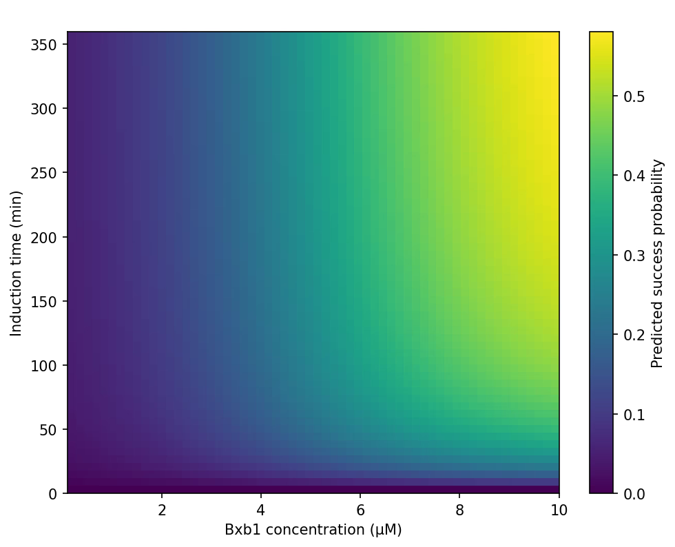
This analysis revealed a broad plateau where φtot becomes insensitive to both induction time and enzyme concentration. Specifically:
- φtot rapidly increases during the first 20–30 minutes,
- and saturates for 0.3–1.0 μM Bxb1,
- with almost no additional gain beyond 30 minutes.
This explains why:
- Mode B predictions are weakly dependent on Bxb1 concentration,
- A standard 30-min induction reliably reaches functional enzyme levels,
- The protein-layer term in M5 can be represented by a single normalization factor fprot.
Supports: Protein sufficiency factor (fprot).
Trend 2 — DNA Layer (M3): Replication Timing × GC% Map
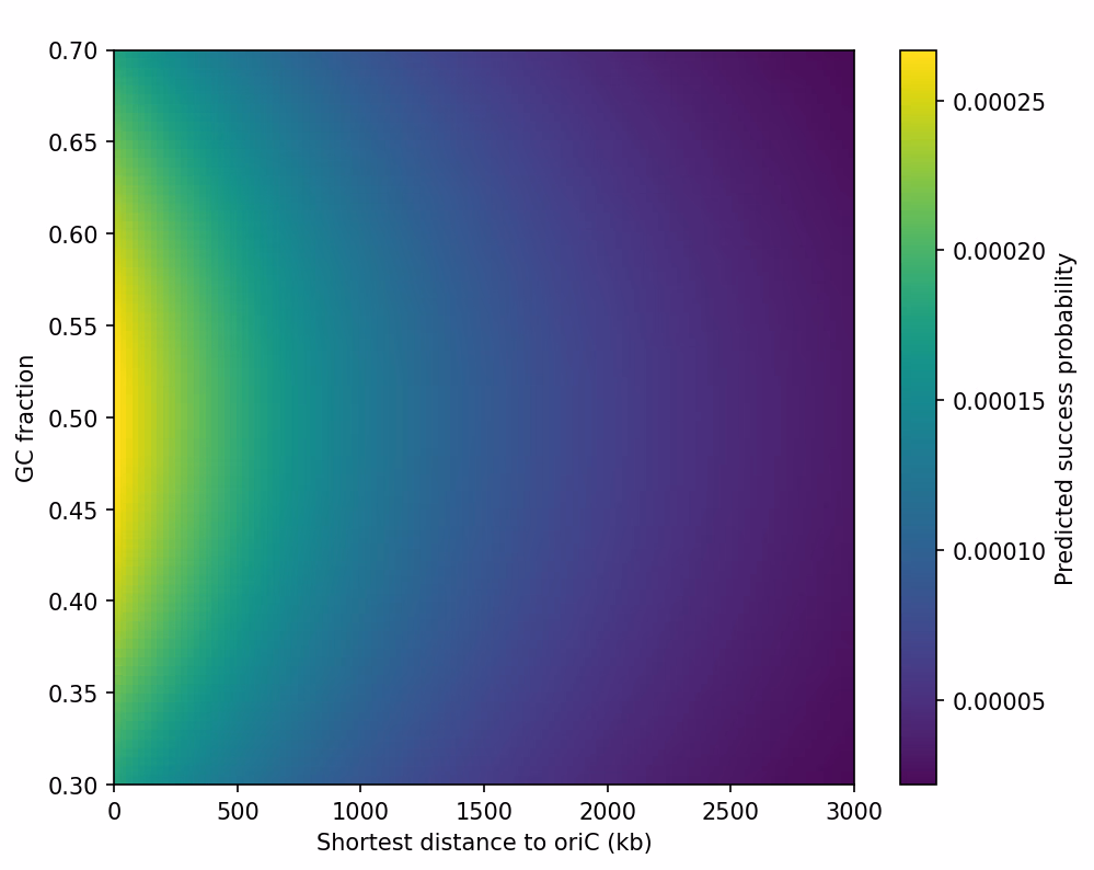
Single-cell stochastic simulations showed two strong effects:
-
oriC–ter replication gradient
- Loci closer to oriC display sharply higher attB-installation probability.
- Efficiency drops ~10–20× toward the terminus.
-
GC% penalty
- GC extremes (<40% or >65%) reduce oligo survival and pairing probability.
- A mild optimum appears near ~50% GC.
These two effects were highly consistent across parameter perturbations, providing the mechanistic basis for incorporating genomic position and GC stability as explicit factors in M5.
Supports: fpos (locus effect), fGC (GC penalty).
Trend 3 — Geometry (M4): Spacer × Insert Length Synergy
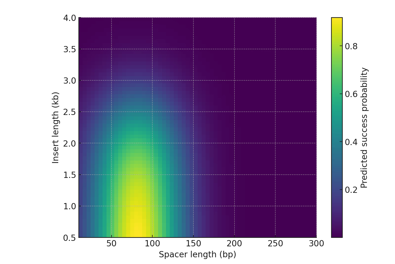
M4 simulations revealed a geometric optimum for dual-end capture:
- A broad maximum occurs at ~60–100 bp spacers,
- Very short (<40 bp) or long (>150 bp) spacers disrupt synapsis,
- Insert length introduces a monotonic penalty, becoming dominant above 2 kb.
This trend provides the structural justification for:
- Treating spacer as a geometry-specific factor,
- Treating insert length as a global multiplicative penalty, and
- Using the limiting-end principle for two-site recombination.
Supports: fdist (length + spacer geometry).
Trend 4 — Length-Penalty Curve (M4): Dominance of Insert Size
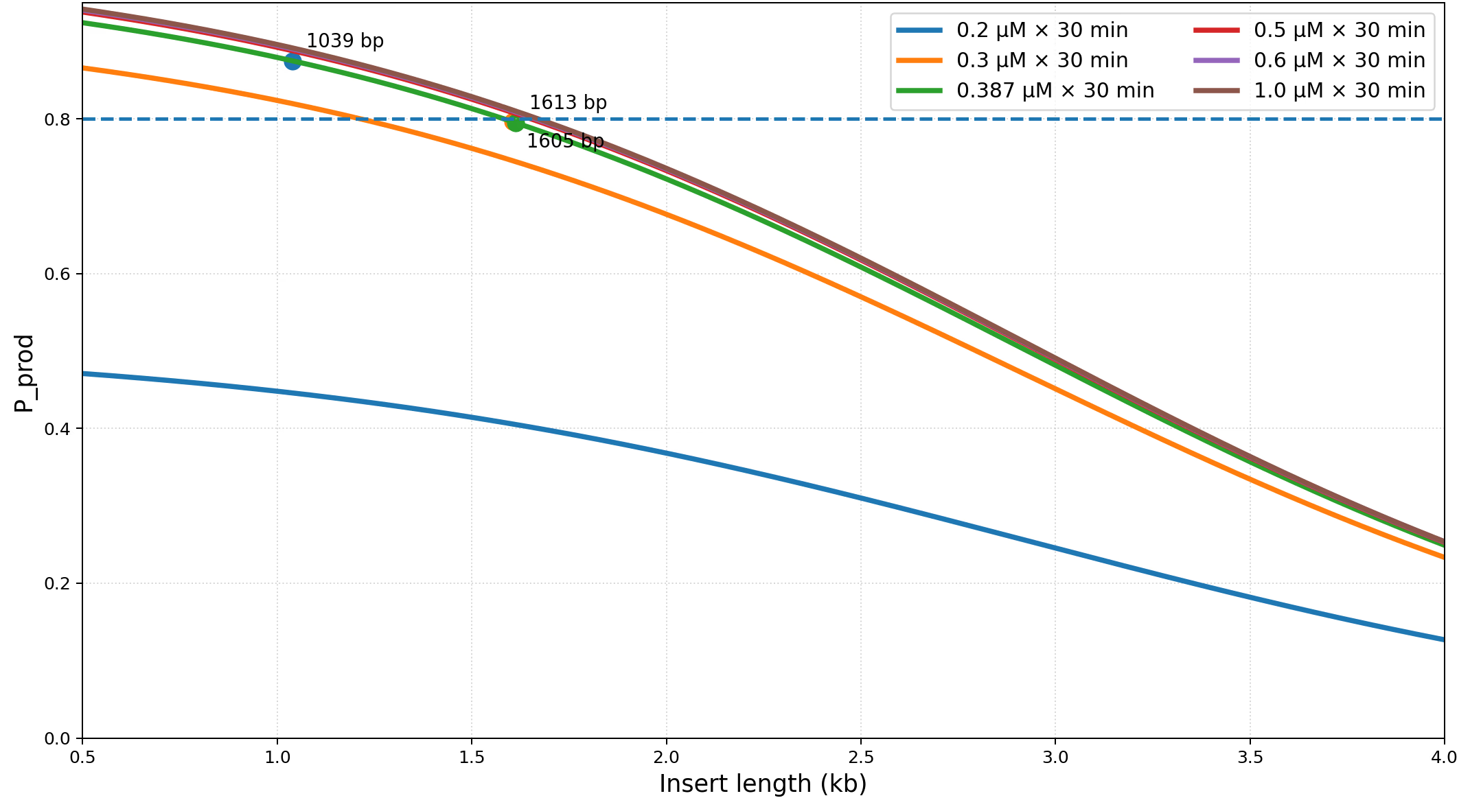
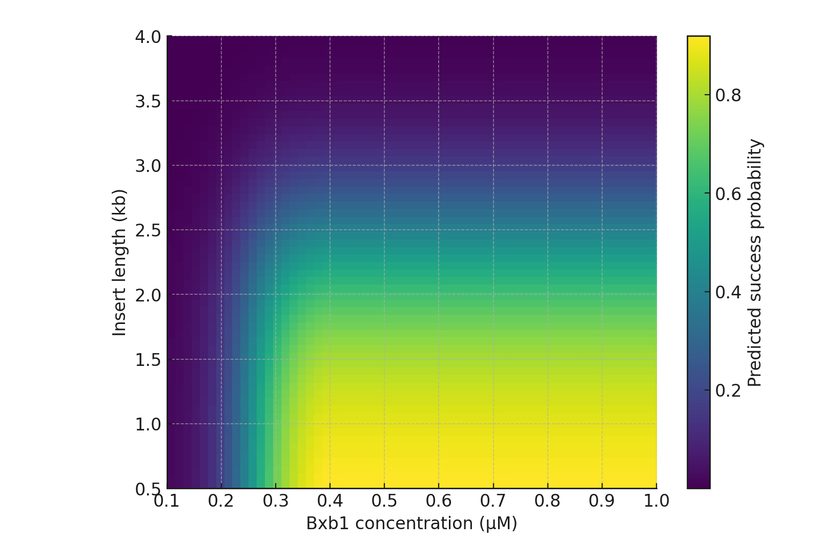
A striking observation across M4 is that:
- Length dictates 90–95% of the variance in Mode B,
- Concentration sweeps converge onto nearly identical curves,
- Experimental validation points fall directly on the predicted curve.
This validated the use of a logit-linear length penalty inside M5 and supported the engineering claim that insert length is the primary determinant for Mode B efficiency.
Supports: fdist (dominant length effect).
Trend 5 — Population Layer: Uptake Mean × CV Map
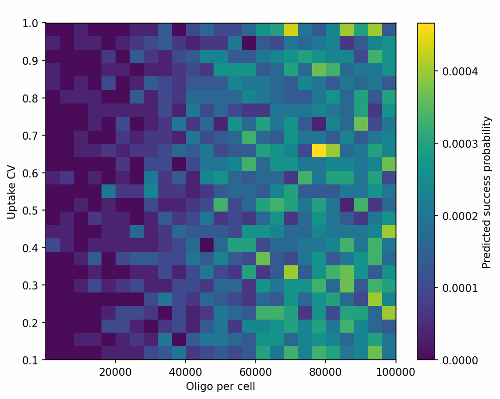
M3–M4 propagation into M10k-scale population simulations revealed:
- Low mean uptake limits the available attB precursor pool.
- High CV amplifies left-tail events where a large subpopulation receives almost no oligo.
- These effects are mode-dependent: strong for Mode A, marginal for Mode B.
This justified the inclusion of the population-level scaling factor α, which differentiates the two integration modes.
Supports: α (population correction for Mode A/B).
Trend 6 — Steric Kinetic Factors (M4): kf2 × krel Sensitivity
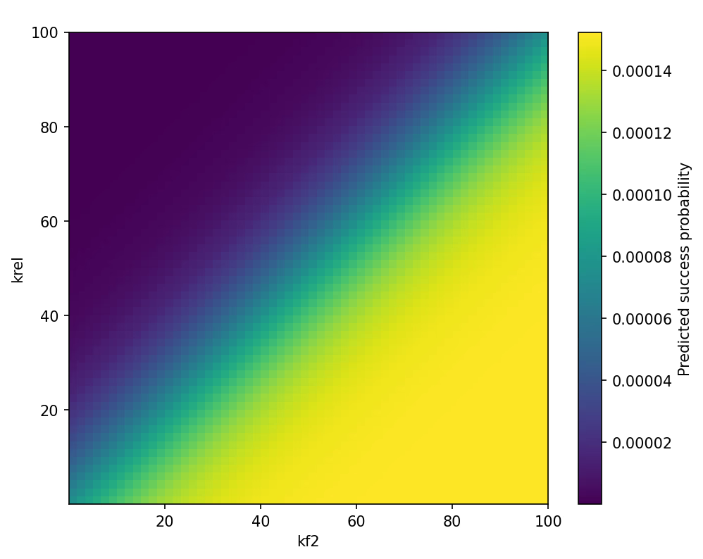
While not directly tunable during experiments, sensitivity analysis showed:
- Length penalties emerge naturally in regions where synapsis formation slows (kf2↓)
- or release becomes rate-limiting (krel↑).
This validated that the geometry/length effects in M5 do not require ad-hoc curve fitting, but arise from fundamental kinetic asymmetry.
Supports: Mechanistic plausibility of fdist and orientation factor.
Trend 7 — CFU → Expected Positive Colonies
This mapping connects:
- single-cell probability (Pfinal)
- → population outcome (expected positives)
This trend allowed M5 to integrate with the software’s AI suggestion system (e.g., advising additional plates if uptake is poor).
Supports: Population interpretation of Pfinal.
(Cite as: “All equations and parameter values correspond to the M5 model internal specification.”)
This section documents all mathematical formulations, parameter values, and computational rules used to generate the M5 heatmaps (Figures 1–8).
These details are not required in the main Model page but are provided here for transparency, reproducibility, and cross-strain recalibration.
C.1 Mode B — Core Predictive Model (Production Mode)
1. Logit–Linear Length Model
Used in Fig. 1, Fig. 2, Fig. 3, Fig. 7.
$$\operatorname{logit}(P_{\text{base}})= a - bL$$ $$P_{\text{base}}=\frac{1}{1+\exp[-(a-bL)]}$$
Parameters (calibrated from experimental anchors):
Symbol | Value | Notes |
|---|---|---|
$a$ | 3.0161 | Defined by 1039 bp → 87.5% |
$b$ | $$ 1.03\times10^{-3},{\rm bp^{-1}} $$ | Joint fit from 3 anchors |
2. Concentration Normalization (Hill Function)
Used in Fig. 1–2.
$$f_{\text{conc}}(C)= \frac{C^n}{K^n + C^n} \bigg/ \frac{C_{\text{ref}}^n}{K^n + C_{\text{ref}}^n}$$
Parameters:
Symbol | Value | Notes |
|---|---|---|
$K$ | 0.20 μM (200 nM) | Local half-saturation |
$n$ | 6 | Steep plateau slope |
$C_{\text{ref}}$ | 0.387 μM (387 nM) | Standard operating concentration |
3. Final Output Rule (Production Probability)
$$P_{\text{prod}} = \min(P_{\text{base}} \cdot f_{\text{conc}} , 0.95)$$
A soft cap at 0.95 prevents overconfidence in high-L extrapolation.
4. Population-Level Output (Fig. 3)
$$E[\text{positive colonies}] = N_{\rm CFU} \times \min(\alpha_{\rm pop} P_{\text{prod}},1)$$
Parameters:
Symbol | Value | Description |
|---|---|---|
$N_{\rm CFU}$ | 10–40 | Colonies plated |
$\alpha_{\rm pop}$ | 1.0 (default) | Transformation amplification factor |
C.2 Mode A — Genomic Site-Selection Maps (First-Round Integration)
Used in Fig. 4 & Fig. 5.
1. Distance-from-oriC Effect
$$F_{\text{distance}}(d) = \exp(-k_d d)$$
Symbol | Value | Notes |
|---|---|---|
$k_d$ | $7\times10^{-4},{\rm kb^{-1}}$ | Distance-decay constant |
$d$ | 0–3000 kb | Shortest distance to oriC |
2. GC Content Penalty
$$f_{\text{GC}}(gc)=\exp[-\gamma(gc - 0.5)^2$$
Symbol | Value |
|---|---|
$\gamma$ | 10 |
gc | 0.30–0.70 |
3. Combined DNA-Layer Probability
$$P_{\text{DNA}} \propto f_{\text{GC}}(gc)\cdot F_{\text{distance}}(d)$$
This determines the color scale in Fig. 4 (not an absolute probability).
C.3 Protein-Layer Operational Window (Fig. 5)
$$\phi_{\text{tot}} = \phi_{\text{Bxb1}}(C)\cdot \phi_{\text{time}}(t)\cdot \phi_{\text{ssAP}}(t_{\text{ssAP}})$$
1. Concentration Activation Curve
$$\phi_{\text{Bxb1}}(C)=\frac{C^{n_H}}{C_{50}^{n_H}+ C^{n_H}}$$
Symbol | Value |
|---|---|
$C_{50}$ | 1 μM |
$n_H$ | 1 |
2. Time-Over-Threshold Function
$$\phi_{\text{time}}=\frac{t}{T_{50}+t}$$
Symbol | Value |
|---|---|
$T_{50}$ | 30 min |
3. ssAP Module
$$\phi_{\text{ssAP}}=\frac{t_{\text{ssAP}}}{T_{\text{ssAP50}}+t_{\text{ssAP}}}$$
Symbol | Value |
|---|---|
$T_{\text{ssAP50}}$ | 20 min |
$t_{\text{ssAP}}$ | 45 min (fixed) |
C.4 Population-Layer Heterogeneity Model (Fig. 6)
Each cell receives DNA according to a log-normal distribution:
$$\sigma = \sqrt{\ln(\text{CV}^2 + 1)}, \qquad \mu = \ln(\text{mean}) - \frac{\sigma^2}{2}$$
Single-cell success:
$$P_{\text{cell}} = \min(P_{\text{calibrated}}, G^{\alpha\beta}, \text{uptake},; 0.8)$$
Monte Carlo: 10,000 simulated cells per grid point.
Parameters:
Symbol | Value | Notes |
|---|---|---|
mean | 20k–100k | Electroporation uptake |
CV | 0.1–1.0 | Transformation heterogeneity |
$G$ | 6.632173469 | Global scaling factor |
C.5 Spacer-Length Geometry Module (Fig. 7)
$$ f_{\text{spacer}}(S)=\exp\left[-\frac{(S-80)^2}{2(40)^2}\right] $$
Symbol | Value |
|---|---|
Optimal S₀ | 80 bp |
σ | 40 bp |
Final probability:
$$P_{\text{prod}} = P_{\text{base}}(L), f_{\text{conc}}(C), f_{\text{spacer}}(S)$$
C.6 Mechanistic Steric Map (Fig. 8)
Length-dependent rate modification:
$$k_{f2} \to k_{f2} e^{-\alpha_{\text{mech}}L}$$
$$k_{rel} \to k_{rel} e^{-\beta_{\text{mech}}L}$$
Parameters:
Symbol | Value |
|---|---|
αmech | $8.5\times10^{-4},{\rm bp^{-1}}$ |
βmech | $8.5\times10^{-4},{\rm bp^{-1}}$ |
Global G | 6.632173469 |
Underlying slope matches empirical:
$$\text{SLOPE} = 1.70\times10^{-3},{\rm bp^{-1}}$$
C.7 Master Parameter Table (Consolidated)
(You may include this as a downloadable CSV)
Layer | Parameter | Value | Purpose |
|---|---|---|---|
Mode B (Length) | a | 3.0161 | Intercept |
b | $(1.03\times 10^{-3})/bp$ | Length slope | |
Mode B (Conc.) | K | 0.20 μM | Half-saturation |
n | 6 | Hill coefficient | |
Cref | 0.387 μM | SOP condition | |
Protein Layer | C50 | 1 μM | Global activation |
nH | 1 | Hill | |
T50 | 30 min | Time half-max | |
TssAP50 | 20 min | ssAP kinetics | |
DNA Layer | kd | $7\times10^{-4}/\text{kb}$ | oriC-distance decay |
γ | 10 | GC penalty | |
Mechanistic | G | 6.63 | global scaling |
αmech | $8.5\times10^{-4}/bp$ | Length penalty | |
Population | αpop | 1.0 | plating amplification |
Spacer | S0 | 80 bp | optimal spacer |
σ | 40 bp | width |
Dry-Lab Results
Through the M1–M5 modeling framework, we established an interpretable, quantitative system that deconstructs Bxb1-mediated genome integration into three interconnected layers — protein, DNA, and population.
Both simulations and experimental data consistently revealed that integration success is not determined by a single kinetic parameter, but by the combined influence of replication timing, DNA geometry, and protein expression dynamics.
1. Locus Effect Dominates (Replication Timing)
Integration efficiency exhibited a clear hierarchy across genomic loci: hisA and metA achieved the highest success rates, galK showed intermediate performance, while leuD and lacZ were markedly lower.
This gradient mirrors the loci’s relative distance from oriC, indicating that replication fork timing is the primary determinant of integration efficiency.
Regions near oriC are duplicated early and remain more accessible to recombineering enzymes, whereas loci near ter replicate later, limiting accessibility.
Notably, lacZ is physically positioned near hisA and galK, not in the terminal region. Its low success rate—comparable to leuD—stems from its two-to-two configuration, which requires recombination across two pairs of attB/attP sites, unlike the single pair used in one-to-one designs.
This contrast reveals that integration efficiency is shaped not only by replication timing but also by geometric coordination within the DNA architecture.
2. Geometry as a Limiting Factor
In a one-to-one configuration, recombination proceeds independently at a single attB/attP pair.
By contrast, the two-to-two configuration demands synchronized recombination at both ends, introducing challenges in molecular alignment and spatial coordination.
Our model predicts that if one end completes recombination prematurely, Bxb1 molecules may become transiently trapped at that site, leading to temporal asymmetry and stalling of the opposite reaction.
This explains the lower initial efficiency observed for lacZ, which reflects geometric instability rather than locus position.
3. Turning Geometry into Advantage — The Strength of Two-to-Two Integration
While the two-to-two configuration introduces additional geometric constraints, it uniquely enables full cassette integration within a single step, a feat impossible for one-to-one architectures.
Our simulations revealed that the inefficiency of dual-end recombination is not intrinsic to the mechanism but results from unoptimized parameters such as inter-site spacing, enzyme concentration, and induction timing.
Once these were optimized in the M5 framework, the predicted success rate of two-to-two events converged with that of one-to-one integrations.
This finding redefines two-to-two recombination as a design-driven advantage rather than a structural limitation.
By quantifying geometric coordination, the model transforms a former bottleneck into a high-performance, scalable solution for production-level genome engineering — proving that dual-end integration can be both complete and efficient when designed systematically.
4. Distinction Between the First and Second Two-to-Two Rounds
The first two-to-two process (installation of dual attB sites) and the second two-to-two process (dual-end cassette integration) represent distinct mechanistic stages.
The first is probability-limited, governed by ssAP expression level and replication-fork timing, resulting in a very low success rate (~0.00195%).
The second occurs only in cells already containing dual attB sites; it is kinetics-limited, dominated by Bxb1 binding and catalytic efficiency.
Under optimized conditions (0.3–1.0 μM Bxb1 and short inter-site spacing), integration proceeds rapidly, reaching success rates exceeding 80%.
This dramatic contrast marks a shift from probabilistic to kinetic limitation, clarifying why integration efficiency can increase by four orders of magnitude between the two stages.
5. DNA Length Defines an Efficiency Window
Insert length strongly affects dual-end recombination success.
Both simulations and experiments show that fragments of 1–2 kb yield consistently high efficiencies, while inserts longer than ~3 kb result in a sharp decline.
This pattern reflects a trade-off between reaction kinetics and molecular proximity: longer fragments reduce the likelihood that both ends align simultaneously, thereby lowering the probability of complete integration.
Thus, insert length emerges as a highly tunable design parameter in optimizing two-to-two architectures.
6. Protein Timing Raises the Integration Ceiling
The M1–M2 models predict optimal induction durations of ≈45 minutes for ssAP and ≈240 minutes for Bxb1. When residual transcription during the cooling phase was incorporated, the simulated protein accumulation curves matched experimental observations. These results show that fine-tuning expression timing determines the achievable “integration ceiling”: operating within the predicted windows significantly increases both attB formation and total integration success.
7. Population-Level Heterogeneity Explained by Replication Gating
The M3 model simulates attB formation as a stochastic single-cell event and successfully reproduces the experimentally observed “polarized” outcomes, where most cells fail to integrate while a minority succeed. This heterogeneity arises from replication-fork gating: integration occurs primarily during the brief window when the replication fork passes through the target locus, rendering DNA temporarily accessible to ssAP-mediated recombination. Replication timing, therefore, is the underlying driver of both population heterogeneity and the oriC–ter efficiency gradient.
8. Integration of All Layers — From Model to Design Assistant
Together, these models define three interacting principles:
The M5 model, implemented as our open-source software GenOMe Navigator, integrates these three layers into a predictive design assistant. Users can input locus position, insert length, and induction schedule to estimate integration efficiency and receive quantitative SOP recommendations, transforming experimental planning from trial-and-error into rational, data-driven design.
9. Future Refinements
While the M5 framework already reproduces experimental trends with strong fidelity,several refinements could further elevate its predictive precision:
- Expanding locus-level replicates to enhance statistical robustness;
- Incorporating direct replication-timing data instead of inferred positions;
- Refining geometric loss modeling for complex two-to-two architectures;
- Automating parameter calibration across experimental batches.
These extensions represent next-generation upgrades rather than current limitations— laying the foundation for M5 to evolve into a fully predictive genome-design platform.
10. Summary
Integration of modeling and experimental data yields the following key insights:
Integration efficiency follows an oriC-to-ter gradient defined by replication timing.
Two-to-two geometry, once optimized, achieves high-efficiency dual-end recombination comparable to one-to-one events.
The first and second two-to-two rounds are governed by distinct kinetic bottlenecks — the former by attB formation probability, the latter by enzymatic and geometric factors.
A 1–2 kb length window represents the optimal trade-off between completeness and efficiency.
Protein induction timing defines the integration ceiling.
The M5 model (GenOMe Navigator) converts these multilayer rules into a reproducible, quantitative, and design-driven framework for genome engineering.
In essence, integration success emerges from the interplay of timing, geometry, and kinetics.
The locus provides opportunity, the geometry sets boundaries, and protein dynamics determine attainment.
Through calibrated modeling, these elements are unified into a single predictive platform — transforming genome integration from empirical trial-and-error into a rational, engineering discipline.
