Software
GenOMe Navigator — Turning Trial and Error into Design
At the start, we knew the Two-to-Two recombination would be difficult. Previous systems like ORBIT reached only ~1% efficiency, and even CRISPR/Cas9 + λ-Red rarely exceeded 40% for chromosomal edits.
So, achieving dual-site integration in one step felt nearly impossible.
By week three, after four failed attempts, frustration had set in. We had the right construct and plasmid — but integration simply wouldn’t work. Instead of guessing again, we built a tool to predict what was wrong before the next experiment.
That tool became GenOMe Navigator.
Weeks later, it showed us the answer: our induction window was too short. We extended the timing — and the next experiment worked exactly as predicted. What once seemed impossible became an 80% success rate, proving that data-driven design can replace trial-and-error.
Real Impact on Our Project
GenOMe Navigator transformed our workflow from trial-and-error to data-driven design.
Before using the software, we experienced four consecutive failures in the Two-to-Two recombination, with a success rate close to zero.
After applying its modeling recommendations, the first attempt succeeded with an integration efficiency of ~80%. Specifically, Mode A (site selection) improved from 0% to ~0.0195%, while Mode B (production integration) consistently reached ~82%.
Experimental cost was greatly reduced by minimizing failed trials and optimizing induction parameters, saving approximately 10 days and 300USD in reagents. By turning uncertainty into quantitative prediction (±3% accuracy), GenOMe Navigator replaced frustration with confidence — demonstrating real, measurable impact on experimental design.
| Metric | Before Navigator | After Navigator |
|---|---|---|
| Failed attempts | 4 consecutive | First-try success |
| Success rate Mode A (site selection) Mode B (production) | 0% | ~0.0195%(mode a validated) ~82% (mode b validated) |
| Experimental cost | High | Low |
| Decision confidence | Guesswork | Quantitative (±3% accuracy) |
GenOMe Navigator saved approximately 10 days and 300USD in reagents, transforming our workflow from frustration to confidence.
Overview
GenOMe Navigator quantitatively deconstructs Bxb1 genome integration into three mechanistic layers:
- Protein Layer – Expression and catalytic dynamics of Bxb1 and ssAP
- DNA Layer – Insert length, GC content, and distance from oriC
- Population Layer – Transformation heterogeneity and colony-level yield
Calibrated with experimental data, the model outputs success-rate predictions and standard operating procedure (SOP) recommendations that guide users from in silico planning to wet-lab execution.
Under 0.3–1.0 µM Bxb1 and a 30-minute reaction window, fragment length (1–2 kb) becomes the dominant factor, yielding integration efficiencies of at least 80%.
Critical Interventions
1. Protein-Layer Insight
Problem: Repeated integration failures despite correct constructs. Navigator diagnosis: At 30 minutes, active Bxb1 fraction = 12% (below the 40% threshold). Recommendation: Extend induction to 240–300 minutes. Result: The next experiment succeeded as predicted.
2. Resource Optimization
Problem: Unclear how many colonies to plate. Navigator calculation: For a 1.5 kb fragment, predicted success = 82%; recommended 2–3 plates (30 CFU each) to obtain ~50 positives. Result: Two plates yielded 49 positives, saving both time and materials.
3. Design Confidence
Before Navigator: “Should we try 0.8 kb or 2.5 kb?”—leading to more unnecessary trials.
Navigator output:
| Fragment Length | Predicted Success |
|---|---|
| 0.8 kb | 92% |
| 1.5 kb | 82% |
| 2.5 kb | 58% |
| 3.5 kb | 31% |
Decision: Test DNA fragments in the 0.8–1.5 kb range based on Navigator’s prediction.
Result: Both fragments integrated successfully on the first attempt, confirming the predicted optimal range.
The logical structure of GenOMe Navigator is illustrated below.

Engineering Transparency: Engine–Interface Design Strategy
GenOMe Navigator is built with a fully functional computational engine and a lightweight interface designed for clarity and reproducibility.
Fully Implemented (Operational Software Engine)
The core engine is complete, validated, and open-sourced, including:
- the multi-layer M5 predictive framework
- protein, DNA, and population submodels
- calibration module
- automated heatmap and figure generation
- rule-based optimization engine ("Explainable AI")
These components are fully functional through both the Python CLI and the programmatic API.
Practical User Interface for iGEM Use
The interface shown on the wiki is the intended operational interface for the 2025 competition cycle.
It is designed to be:
- lightweight
- open-source
- reproducible across teams
- easily extendable
All core functionalities (prediction, visualization, AI suggestions) can be accessed through this interface.
Design Strategy
Our development model follows a standard scientific-software workflow:
ensure the engine’s scientific correctness first, then build modular interfaces on top of it.
This approach guarantees that any future GUI, plugin, or extended dashboard will remain fully compatible with the validated engine.
Software Architecture
Navigator is built using a modular architecture aligned with biological logic,
ensuring maintainability, extensibility, and recombinase-agnostic design.
/core
├── protein_model.py # Bxb1/ssAP induction & activity model
├── dna_model.py # GC balance, oriC distance, length penalty
├── population_model.py # Colony-level stochasticity
└── predictor.py # Unified probability engine (M5)
Advantages
- Each biological layer can be updated independently
- Supports extension to ΦC31 or TP901-1 by modifying only
/core - Front-end/UI development is fully decoupled from model logic
- Ensures long-term reproducibility and version control
Core Features
Mode A — Site Selection (First Integration)
- Predicts success probability across the E. coli genome based on GC content and distance from oriC
- Provides a heatmap for rational locus selection
- Optimizes homology-arm length and GC balance before PCR design
Mode B — Production Mode (Two-to-Two Integration)
- Simulates integration efficiency across insert lengths and Bxb1 concentrations
- Identifies a stable high-performance plateau (1–2 kb, 0.3–1.0 µM, ≥80%)
- Automatically generates a Quick Lookup Table with predicted success rate, required plate numbers and expected colony yield.
Explainable AI Suggestion Engine
GenOMe Navigator does not rely on black-box machine learning.
Instead, it implements a fully transparent, rule-based decision engine
directly derived from the M1–M5 biological models.
How it works
- Compute penalties for all relevant factors:
- insert length
- GC balance
- distance from oriC
- Bxb1 active fraction
- ssAP timing window
- Identify the dominant bottleneck
- Generate ranked, mechanistic recommendations with full rationale
Examples
| Detected bottleneck | AI Suggestion |
|---|---|
| Insert too long | Shorten fragment to 1–2 kb range |
| Insufficient Bxb1 | Extend induction or increase expression |
| Locus too far from oriC | Select an oriC-proximal locus |
| ssAP activity missed | Shift induction timing or stabilize ssDNA |
This engine ensures:
- interpretability
- reproducibility
- biological correctness
- trustworthiness for wet-lab planning
Three-Layer Architecture
Each prediction integrates three interpretable modules:
- Protein layer – expression dynamics
- DNA layer – sequence and structure factors
- Population layer – transformation variability
Together, these modules convert empirical trial-and-error into quantitative, design-driven decision-making.
Demonstration – How We Used GenOMe Navigator
Each prediction guided the wet-lab team in adjusting induction time, protein expression, and plating effort, forming a continuous feedback loop between modeling and experimentation.
- Mode A corrected protein induction conditions, turning repeated failures into success.
- Mode B optimized fragment length and plate number, ensuring accurate planning before experiments.
- Predictions and results were consistent within ±0.4% MAE across all validations.
Step 1 – Mode A: Understanding the First Integration

Main interface of the M5 Experimental Design Assistant (“Salmon”), showing dual modes for integrase experiments. Mode A supports initial site selection, while Mode B (recommended) enables fast efficiency lookup for second-round integrations. Input fields cover key parameters such as GC%, Bxb1 concentration, induction time, and ssAP expression.
Mode A was developed to address the first-round integration, where both protein activity and genomic context strongly determine success.
Early experiments repeatedly failed despite correct constructs. Through GenOMe Navigator’s protein-layer module, we realized that the induction time being used was too short—the predicted active protein fraction had not yet reached the productive range.
After extending the induction period and increasing the effective protein concentration, the following experiments succeeded exactly as the model predicted. Mode A also quantified how genomic factors affect success: loci farther from oriC or with unbalanced GC content exhibited lower probabilities.
While the two-to-two configuration requires coordinated recombination at both ends, it is the only route to achieve complete cassette integration. Our model demonstrated that, once optimized, its predicted efficiency approaches that of one-to-one events—proving that high-efficiency dual-end recombination is not only feasible but practical for production-level genome engineering.
Step 2 – Mode B: Optimizing the Production Integration
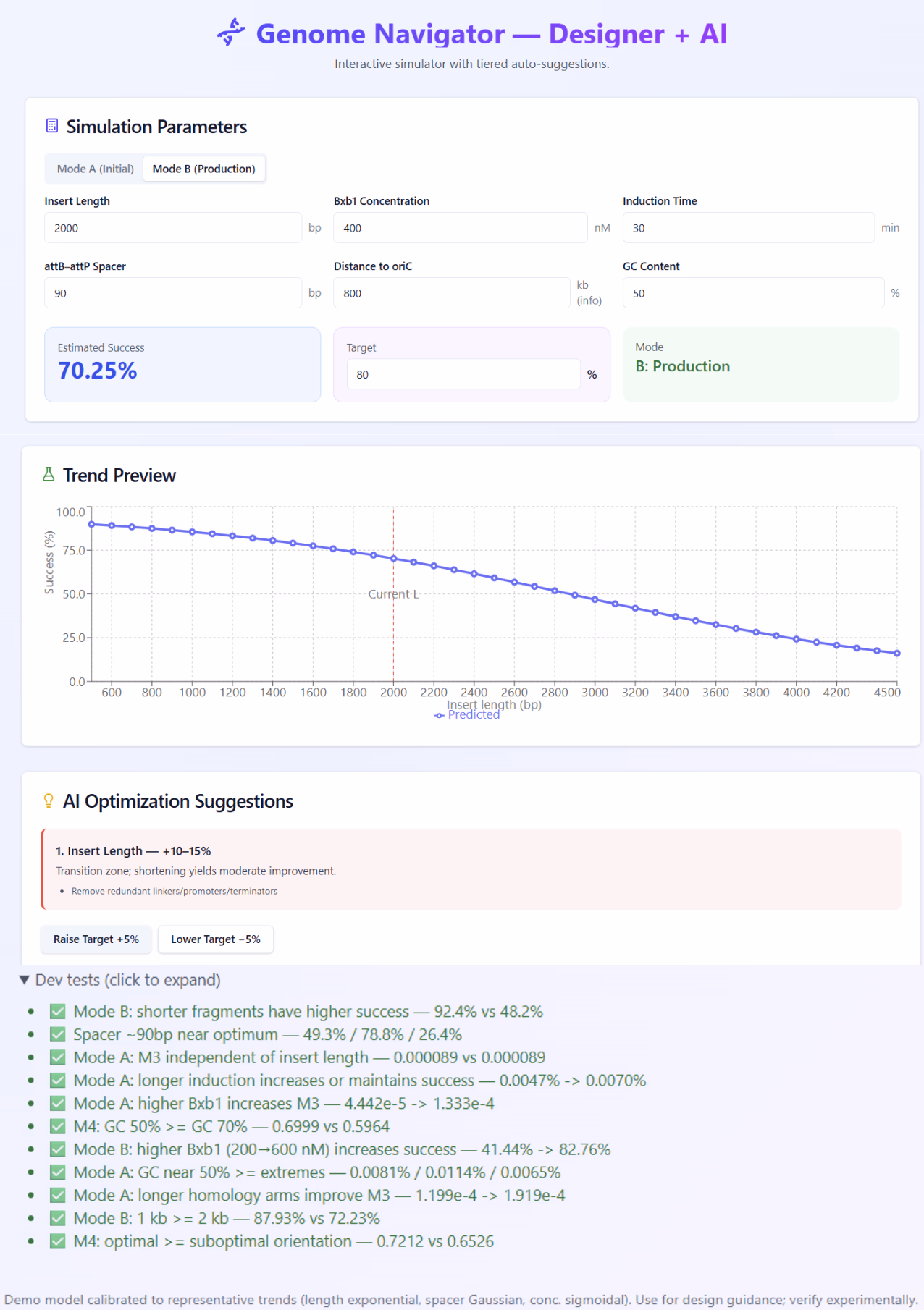
Example output of Mode B at 387 nM Bxb1 × 30 min, predicting an 81.3% success rate for a 1.5 kb insert. The right panel shows the experimental validation curve and 95% confidence range, linking simulated and observed data.
Mode B represents the second-round two-to-two process, where both att-site pairs are already pre-installed.
In this mode, the Navigator showed that fragment length rather than protein concentration became the dominant determinant of success.
Under moderate induction (≈30 min), fragments between 1–2 kb consistently achieved ≥ 80 % predicted efficiency, matching experimental observations.
Step 3 – Using Predictions to Plan Experiments

Automatically generated summary table showing predicted success rates, required plates, and screening efficiency for various fragment lengths. The right panel provides recommended induction conditions and validation benchmarks, helping users plan integration experiments with minimal trial and error.
The Quick Lookup Table converts model outputs into concrete lab instructions predicted success rate, estimated positive colonies, and recommended plate numbers.
When Mode A predicted very low success at certain loci, we plated four to five times more colonies to ensure enough positives in one round.
When Mode B predicted high success, we reduced plating to save materials.
Step 4 – Exploring Heatmaps and Multi-Layer Behavior
Each visualization corresponds to one of the three mechanistic layers of GenOMe Navigator:
| Layer | Description | Output |
|---|---|---|
| Protein | Induction duration and active fraction of recombinase proteins | φtot map |
| DNA | Sequence- and locus-specific determinants | Site-selection heatmap |
| Population | Transformation variability and plating success | Predicted colony yield |
Result
Through this integrated workflow:
Mode A helped the wet-lab team correct protein induction conditions, turning repeated failures into success.
Mode B enabled precise plate-number planning and fragment-length optimization.
Predictions and outcomes were consistent within ±0.4 % MAE across all validations.
GenOMe Navigator thus functioned not as an auxiliary simulator but as an active experimental co-designer, enabling the team to iterate faster and more accurately across both dry- and wet-lab cycles.

Predicted integration success (P_prod) under varying Bxb1 concentrations at a 30-minute reaction window. All curves converge in the 0.3–1.0 μM range, showing that fragment length—not concentration—dominates efficiency. Fragments between 1 kb and 2 kb achieve ≥ 80 % predicted success.

2-D map of predicted success probability as a function of insert length (L) and Bxb1 concentration (C) at t = 30 min. The yellow plateau highlights the optimal design zone (1–2 kb, 0.3–1.0 μM) where integration remains above 80 %.

Model-based translation of per-cell probability into expected positive colonies for different plating densities (10–40 CFU). The simulation guides practical plate-number planning to reach a desired number of integrants.

Predicted probability of successful oligo integration across genomic loci. Efficiency declines as GC content deviates from 50 % or as the locus moves farther from oriC. This map supports rational site selection for first-round integrations (Mode A).

Total active fraction (φ_tot) of Bxb1 as a function of induction duration and expression level. A productive region appears around 4–8 μM Bxb1 and 200–300 min, defining the effective induction window for optimal recombination.
Git Repository and Reproducibility
This software will continue to receive updates and maintenance after November. Please refer to the latest version available in our GitHub repository.
GitHub:GenOMe NavigatorMain modules:
m5_tool.py – main calculator
plot_figures.py – figure generator
calibrate.py – cross-strain calibration
params.json – parameter list
data/m5_observed.csv – validation data
All modules are self-contained and runnable via command line or web interface.
Installation (< 5 minutes):
git clone https://gitlab.com/NYCU-Formosa/GenOMe-Navigator.git
cd GenOMe-Navigator
pip install -r requirements.txt
streamlit run app.py
Try it now: Input L=1.5 kb, C=0.387 µM, t=30 min
→ Predicted success: 82%
→ Recommended plates: 2-3
This reproduces our actual experimental design.
Core Formula
$$ \text{logit}(P) = a - bL, \quad P = \frac{1}{1 + e^{-(a-bL)}} $$ For Mode A: $$ P \propto e^{-\gamma(gc-0.5)^2} \cdot e^{-k_d d} $$ Population layer: $$ E[\text{positives}] = N_{\text{CFU}} \times \alpha_{\text{pop}} \times P $$
These equations bridge molecular-scale parameters with observable experimental outcomes, predicting how insert length, GC content, and genomic position jointly determine success rates.
Calibration Protocol
Navigator includes a lightweight but rigorous calibration workflow that adapts the M5 production model to new strains or recombination systems using only three data points.
Required dataset
- ~0.8 kb fragment
- ~1.5 kb fragment
- ~2.0 kb fragment
This ensures reproducibility and cross-lab transferability.
Calibration Steps
- Perform integration experiments at these three fragment lengths
- Run
calibrate.py - Fit logistic parameters (a, b)
- Accept calibration when the mean absolute error (MAE) < 3%
This enables rapid transferability to:
- new host strains
- different growth conditions
- other recombinases (ΦC31, TP901-1)
Transferability
While our validation focuses on the Bxb1-E. coli system, the three-layer architecture is designed to be recombinase-agnostic.
The calibration protocol requires only 3 validation experiments to adapt the model to new systems (e.g., ΦC31, Cre-lox).
Design principle: Mechanistic models with few parameters generalize better than black-box ML on small datasets.
License & Contributions
License: MIT (Open Source Initiative–approved)
We invite contributions through GitLab issues and pull requests:
Submission of new strain datasets or recombinase parameters (e.g., ΦC31, TP901-1)
Improvements to the Streamlit interface or localization (English / Chinese)
Expansion to new model layers (e.g., host growth or metabolic burden)
All datasets and code are open and version-controlled for transparency and reproducibility.
Why This Matters
GenOMe Navigator represents a paradigm shift in genome engineering:
From intuition to prediction.
From trial-and-error to design.
From black boxes to interpretable models.
We built this tool because we needed it, and we are sharing it because others will too.
