External: Reusable Modeling Pipeline for Future Teams

To quantify and predict the performance of our system, we developed a comprehensive software pipeline. This tool automates the entire workflow from raw experimental data to a sophisticated system simulation with uncertainty analysis, and we have packaged it as a robust, reusable tool for the iGEM community.

The Three-Stage Analysis Pipeline

Our tool transforms raw data into a predictive simulation in three automated stages:

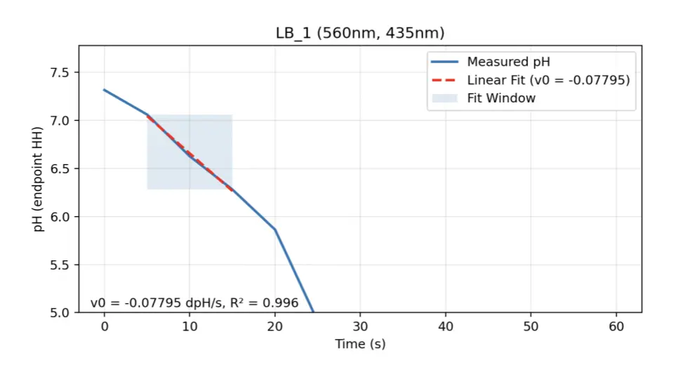
1. Stage 1 (assay): It processes dual-wavelength spectrophotometer absorbance traces (≈560/435 nm) by converting them to pH via the phenol-red ratio and the Henderson–Hasselbalch relationship, identifies an early linear window, and calculates the initial reaction rate \( v_{0} \) along with a data quality score \( R^2 \).



Methods (dual-λ → pH → (\( v_{0} \)))

Ratio: \( R = \dfrac{A_{560}}{A_{435}} \) with endpoints \( (R_{\text{acid}}, R_{\text{base}}) \).

pH transform: \( \mathrm{pH} = pK_a' + \log_{10}\!\left(\dfrac{R - R_{\text{acid}}}{R_{\text{base}} - R}\right) \).

Early rate: \( v_0 = \dfrac{d\,\mathrm{pH}}{dt} \) (linear fit on the first \( t \) seconds; we report \( R^2 \)).

Molar rate: \( v_0^{\text{molar}} = \beta \cdot \dfrac{d\,\mathrm{pH}}{dt} \) (buffer capacity \( \beta \)).

Details & calibration in repo (params.py, assay_v0.py).

2. Stage 2 (fit): We aggregate per-run initial rates \( v_{0} \) from Stage 1 and pair each with its corresponding substrate concentration (([S])) from run_meta.csv. For each enzyme, we fit the Michaelis–Menten model by nonlinear least squares whenever at least three distinct substrate concentrations are available. To quantify uncertainty, we bootstrap the dataset (resampling runs with replacement, refitting (n = 500) times) and record the parameter distributions,reporting the mean, bootstrap standard error, and 5–95 % confidence intervals. If fewer than three unique substrate concentrations are available, we use the fallback one_point_fixed_Km method: \( K_{m} \) is fixed to a literature value (e.g., 9.3 mM for CA) and \( V_{\max} \) is estimated analytically from the available points, still with bootstrap uncertainty. Each enzyme’s output is written automatically to results/kinetics_.json for the user. These fitted parameter distributions feed Stage 3, where the ODE simulator samples \( V_{\max} \)⁡,Km​ to produce personalized predictions with uncertainty bands.

   \( v = \frac{V_{\max}[S]}{K_m + [S]} \)

3. Stage 3 (simulate): It uses these experimentally-derived parameters to power a system of Ordinary Differential Equations (ODEs) that forecasts the system's behavior over time.

A Deep Dive into the ODE Model

The behavior of the system is described by the following set of coupled differential equations:

• \( C_{\text{carb}} \) (mM):

  The concentration of dissolved carbonate.

• \( C_{\text{CaCO3}} \)

  The concentration of precipitated calcium carbonate.

• \( X \)

  The density of viable, productive cells.

The core of our pipeline is a predictive ODE model that simulates the dynamics of biomineralization. The model tracks three key state variables:

\[ \begin{aligned} \frac{dC_{\text{carb}}}{dt} &= r_{\text{prod}} - r_{\text{precip}} \\ \frac{dC_{\text{CaCO3}}}{dt} &= r_{\text{precip}} \\ \frac{dX}{dt} &= \mu_{\text{max}} \cdot \mathrm{burden}(r_{\text{prod}}, V_{\max}) \cdot X \end{aligned} \]

Breaking down each component

1. Carbonate Production \( r_{\text{prod}} \)

The rate of dissolved carbonate production is driven by our engineered enzyme and is modeled using the Michaelis–Menten equation:

\[ r_{\text{prod}} = V_{\max} \cdot \frac{[S]}{K_m + [S]} \]

The parameters \( V_{\max} \) – the maximum reaction rate – and \( K_{m} \) (the substrate affinity) are not assumed; they are derived directly from our wet lab data in the fit stage of the pipeline.

2. CaCO₃ Precipitation \( r_{\text{precip}} \):

   The precipitation of calcium carbonate from solution is modeled using second-order kinetics, dependent on the concentration of both the dissolved carbonate and the available free calcium ions in the media:

   \( r_{\text{precip}} = k_{\text{precip}} \cdot [\text{Ca}^{2+}] \cdot C_{\text{carb}} \)

   Assumptions & Boundary Conditions (for this version of the model)

   • [Ca²⁺] treated as constant and in large excess. We do not deplete calcium in the ODE, so CaCO₃ can increase without a hard stoichiometric cap. This helps visualize kinetics, but in experiments precipitation is capped by the initial calcium pool.
   • Substrate pool is lumped. For CA we treat the CO₂/HCO₃⁻/CO₃²⁻ system as an effective substrate [S] feeding \( r_{\text{prod}} \). Speciation is not explicitly modeled.
   • Well-mixed, isothermal reactor with buffered pH (phenol-red assay).
   • Simple nucleation/precipitation kinetics (second-order in ions); no nucleation lag or polymorph switching.
3. Cell Growth and Metabolic Burden: We moved beyond a simple exponential growth model to more realistically account for the energetic cost of producing our enzyme. The growth rate is modulated by a phenomenological burden factor:

   \[ \text{burden factor} = \left(1 - b_0 - b_1 \cdot \frac{r_{\text{prod}}}{V_{\max}}\right)^{+} \]

   This term dynamically penalizes the maximum growth rate (u_max) based on the cell's metabolic effort. As the enzyme's catalytic flux (r_prod) approaches its theoretical maximum (V_max), cellular resources are diverted, and growth slows. The parameters b0 and b1 represent the basal metabolic burden and the burden from catalytic activity, respectively.

Uncertainty Propagation and Model Predictions

A key feature of our model is its ability to quantify and propagate uncertainty. During the fit stage, we use bootstrapping to obtain parameter distributions for \( V_{\max} \) and \( K_{m} \) (from which we also report 5–95% confidence intervals). The simulate stage then runs hundreds of simulations, sampling from these bootstrap-derived parameter distributions (or perturbing point estimates when distributions are unavailable). The final output plots the mean prediction along with a shaded confidence interval, providing an honest and robust forecast of the system's likely performance range.

A Reusable Tool for iGEM

This entire pipeline is packaged as a user-friendly command-line tool designed for reproducibility. Every run generates a unique, timestamped folder containing all data, plots, parameters, and logs, ensuring that any result is fully traceable. We believe this tool represents a significant contribution that can help future iGEM teams bridge the gap between their wet lab data and predictive modeling.